4 Gross primary production and photosynthesis
In Chapter 3, we conceived the global carbon cycle as a system of three pools (atmosphere, land, ocean), emissions as fluxes into the system (added to the atmosphere), and fluxes between the pools. The C dynamics in the land biosphere were modeled using a 1-box model which receives C inputs through photosynthesis and loses C through a constant turnover. In this chapter, we dive deeper into the processes that drive photosynthetic carbon uptake by land ecosystems.
4.1 Light use efficiency model
Monteith (1972) made the observation that the biomass productivity of a given (well-watered) crop (in the tropics) scales linearly with the amount of absorbed solar radiation, integrated over weeks to months. This observation underlies the general light use efficiency (LUE) model which describes ecosystem-level apparent photosynthesis (referred to as gross primary production, GPP) as the photosynthetic photon flux density (PPFD) and the efficiency at which photons are used for assimilating C (LUE). \[ \mathrm{GPP} = \mathrm{PPFD} \cdot \mathrm{fAPAR} \cdot \mathrm{LUE} \tag{4.1}\] GPP is expressed as a C flux per unit ground area and per unit time (e.g., gC m-2 s-1). PPFD measures the solar radiation flux, incident at the top of the canopy. It is expressed, e.g., in units of mol (photons) m-2 s-1. The light use efficiency model (Equation 4.1) is also often formulated using the photosynthetically active (solar) radiation (PAR) in units of an energy flux per unit ground area (e.g., W m-2), instead of PPFD. This is equivalent to the expression with respect to PPFD, considering that each photon (light quantum) bears a certain amount of radiation energy. fAPAR is the fraction (unitless) of absorbed photosynthetically active radiation. It depends on the total ecosystem-level (or canopy-level) surface area of green leaves (Section 4.2). LUE is the light use efficiency, measuring the efficiency with which photons are harvested and used for assimilating CO2 by the photosynthetic machinery (Section 4.3). It is expressed, e.g., in units of gC (mol CO2)-1. See Table 4.1 for an overview of symbols and abbreviations used in this chapter.
Of course, a relationship with biomass productivity, as observed by Monteith (1972) should not be equated with a relationship with GPP. However, again, over longer periods of time, a plant converts assimilated carbon into biomass at a relatively constant rate (see Chapter 5). Therefore, the observation by Monteith (1972) is instructive for our understanding. Indeed, models of terrestrial GPP are often formulated in the form of Equation 4.1 and are useful for estimating how GPP values over space and time (at the scale of weeks to months). The aspect that the observations by Monteith (1972) were made under well-watered conditions is a further caveat. However, it shall serve us in this chapter as we are–for now–ignoring the effects by limited root-zone water availability. We will relieve this simplification in Chapter 7 and Chapter 8.
The linear dependence of GPP on PPFD implies that the variations of solar radiation over the seasons and across latitude directly translate to how GPP varies across these scales. This will be further described in Chapter 6. Note that at shorter time scales, GPP is no longer linearly related to PAR. Through its influence on GPP, as described by Equation 4.1, solar radiation is the “engine” of photosynthetic CO2 uptake by the terrestrial ecosystems. Temporal and spatial patterns of GPP are strongly driven by patterns in solar radiation. The astronomical mechanics responsible for temporal and spatial (latitudinal) patterns in solar radiation will be introduced in Chapter 6. For now, let’s remember that the incoming (incident) solar radiation is an energy flux that varies strongly over the course of a day and a year. These diurnal and seasonal patterns are different along different latitudes (position north or south of the Equator). In the following, we delve deeper into the two factors fAPAR and LUE in Equation 4.1.
4.2 Canopy light absorption
Photosynthetic CO2 uptake only operates if active (green) leaves are out. The relationship between the amount of leaves and GPP is introduced here. Active leaf area varies across the seasons and space in response to the seasonality of temperature, light and water availability. The seasonal fluctuation of leaf area, most visible for deciduous trees, is referred to as (leaf) phenology. The drivers of temporal and spatial variations of phenology and leaf area are introduced in Section 6.2.
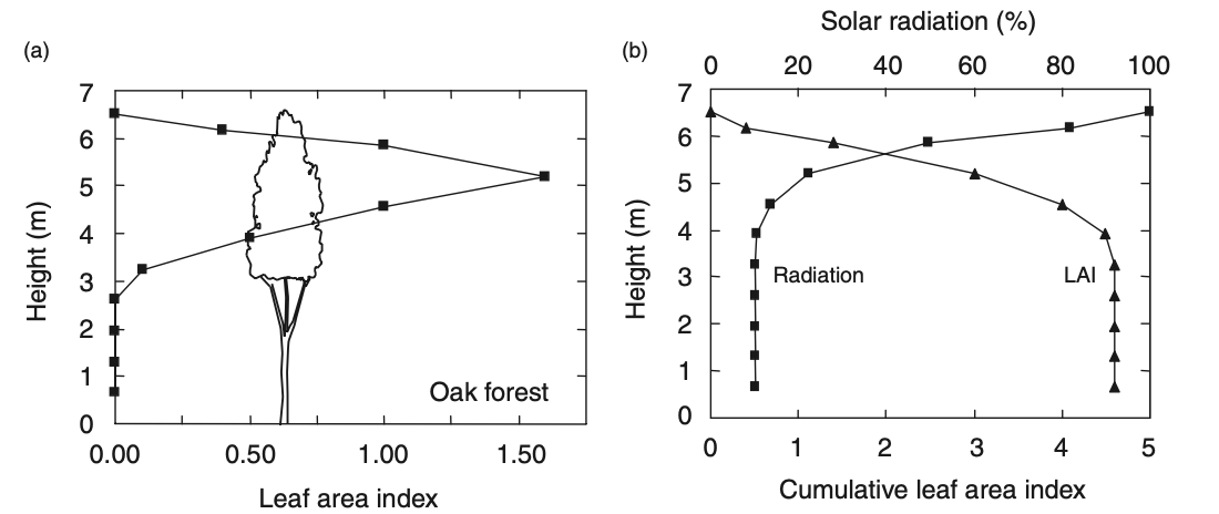
The fraction of absorbed photosynthetically active radiation (fAPAR) increases with the projected (one-sided) surface area of leaves per unit ground area (the leaf area index, LAI). The total surface area of leaves is roughly twice the projected surface area. The LAI is an ecosystem-level variable and reflects the leaf area density of the whole canopy. The canopy may be composed of multiple species and organised in multiple canopy layers (Figure 4.1). While temperate and boreal forests commonly form a single understorey and attain LAI values of 4-6 m2 m-2, tropical moist forests may have multiple canopy layers and an LAI of over 6 m2 m-2 (Figure 2.16).
While the intensity of shortwave (solar) radiation is highest at the top of the canopy, it is progressively attenuated as it penetrates into the canopy. Radiation gets reflected, absorbed and transmitted by individual leaves. The penetration of radiation into a canopy is referred to as canopy radiative transfer. Each of the processes–reflection, absorption, and transmittance–affects light differently in different wavelengths, depends on the solar zenith angle, on the three-dimensional arrangement of leaves in the canopy (angles, “clumping”), and on the pigments on the leaf surfaces that are responsible for light absorption. Pigments change across species and may vary in response to stress (e.g., by frost, heat, or water limitation).
In brief, canopy radiative transfer is complex. A simple model for how (solar) radiation (light) is attenuated as it penetrates into the canopy is given by the Beer-Lambert law. To apply it for canopy radiative transfer, we assume that a leaf only absorbs light, but does not reflect or transmit it. Following this model, the light intensity \(I\) at the bottom of the canopy (\(z_0\)) is an exponential function of LAI (\(L\)). The rate of decline of the light intensity is given by the light extinction coefficient \(k\). A typical value of \(k\) in the visible (photosynthetically active) wavelength spectrum is 0.5. \[ I(z_0) = I_0 \; e^{-kL} \] We have assumed that no light is reflected. Therefore, the reduction of light levels at the bottom of the canopy tells us how much light was absorbed by the canopy (and used for photosynthesis). The fraction of absorbed (photosynthetically active) radiation therefore is \[ \begin{align} \mathrm{fAPAR} &= 1 - I(z_0)/I_0 \\ &= 1 - e^{-kL}\;. \end{align} \]
The shape of this function is illustrated in Figure 4.2 (a). This implies a dependency of light levels on canopy depth \(z\), as illustrated in Figure 4.2 (b) - consistent with the observation shown in Figure 4.1 (b).
Code
library(ggplot2)
library(dplyr)

calc_fapar <- function(lai, k_beer){
  1 - exp(-k_beer * lai)
}

gg_fapar <- ggplot() +
  geom_function(
    fun = calc_fapar,
    args = list(k_beer = 0.5),
    linewidth = 0.75
    ) +
  xlim(0, 10) +
  labs(x = expression(paste("LAI (m"^2, " m"^-2, ")")),
       y = "fAPAR (unitless)") +
  theme_classic()

calc_cumlai <- function(z){
  ifelse(z <= 3.5, z*4.6/3.5, 4.6)
}

calc_light_rel <- function(z, k_beer){
  exp(-k_beer * calc_cumlai(z))
}

df <- tibble(z = seq(0, 7, by = 0.01)) |>
  mutate(
    light_rel = calc_light_rel(z, k_beer = 0.5)
    )

gg_canopydepth <- ggplot() +
  geom_rect(
    aes(
      xmin = 0, xmax = 1,
      ymin = 0, ymax = 3.5
    ),
    fill = "#009E73",
    alpha = 0.5
  ) +
  geom_rect(
    aes(
      xmin = 0.45, xmax = 0.55,
      ymin = 3.5, ymax = 7
    ),
    fill = "sienna",
    alpha = 0.5
  ) +
  geom_line(
    data = df,
    aes(
      y = z,
      x = light_rel),
    linewidth = 1,
    color = "#E69F00"
  ) +
  labs(y = "Canopy depth (m)",
       x = "Light level (relative)") +
  theme_classic() +
  scale_y_reverse()

cowplot::plot_grid(
  gg_fapar,
  gg_canopydepth,
  nrow = 1,
  labels = c("a", "b"),
  rel_widths = c(1, 0.6)
)
TipBasis of the Beer-Lambert law for canopy light extinction
Following the Beer-Lambert law model, the light extinction at canopy depth \(z\) (measuring from the top) is proportional to the light intensity at that depth and an “optical density” \(\mu\). \[ \frac{\mathrm{d}I}{\mathrm{d}z} = -\mu\;I(z) \tag{4.2}\] Therefore, the light intensity declines exponentially with \(z\). \[ I(z) = I_0 \exp(-\mu z) \tag{4.3}\] How does the dependency on \(z\) relate to the dependency on LAI (\(L\))?
For applying the Beer Lambert law, it is further assumed that the canopy is a homogenous turbid medium. In other words, we assume that leaves are uniformly distributed across the canopy and that the optical density is given by the leaf area index \(L\) divided by the total canopy depth \(z_0\): \[ \mu = k \frac{L}{z_0} \tag{4.4}\] \(k\) is the leaf area-specific optical density, or light extinction coefficient. Using Equation 4.3 and Equation 4.4, we can thus express the light level at the bottom of the canopy (\(z_0\)) as a function of \(L\) as \[ I(z_0) = I_0 \; e^{-kL} \] and the fraction of absorbed (photosynthetically active) radiation is \[ \mathrm{fAPAR} = 1 - e^{-kL}\;. \]
The radiation \(I\) consists of direct radiation from the sun and diffuse radiation from the sky and from radiation scattered within the canopy. This distinction is relevant for understanding radiation absorption by the canopy and canopy-level photosynthesis. Two important implications are the following. First, diffuse radiation is more effectively absorbed by canopies, particularly at low LAI. The reduction of GPP under cloudy conditions is therefore less than what would be expected from considering only changes in \(I_0\) (the effective \(k\) is higher for diffuse radiation than for direct radiation).
Second, the energy flux of direct radiation is much higher than that of diffuse radiation. Although at greater canopy depths, leaves are more frequently exposed to diffuse than to direct radiation, the latter provides potentially valuable energy for photosynthesis, but occurs very rarely (sunflecks). Leaves have to balance the rare high-intensity light levels and the frequent low-intensity levels for adjusting photosynthetic capacities.
4.3 Photosynthesis
Light use efficiency (LUE, Equation 4.1) measures the efficiency at which absorbed photons (radiation) are converted into C in the form of sugars. LUE is an ecosystem-level quantity and reflects the collective photosynthetic CO2 uptake efficiency of all leaves in the canopy. This efficiency is determined by the leaf physiology and the activity of the photosynthetic machinery. In this subsection, we dive deeper into the physiology of photosynthesis.
CO2 uptake by the leaf happens by diffusion through pores at the leaf surface (stomata, Figure 4.3). The opening of stomata is dynamically regulated in response to environmental conditions (light, CO2, temperature, atmospheric humidity) and controls the conductance to CO2 diffusion. The CO2 uptake flux by diffusive transport through stomata can thus be described by Fick’s law which states that the flux is proportional to the concentration difference of CO2 inside and outside the leaf. \[ A = g_s(c_a - c_i) \tag{4.5}\] \(c_a\) is the ambient CO2 concentration (outside the leaf), and \(c_i\) is the CO2 concentration inside the leaf–at the chloroplast. \(g_s\) is the stomatal conductance. Note that we use the variable name \(A\) here for CO2 assimilation by photosynthesis. In constrast to the ecosystem-level variable GPP, \(A\) refers to the leaf-level flux.

Once inside the leaf, CO2 diffuses across mesophyll cells to the chloroplasts–the site of photosynthetic reactions. The conductance to this diffusion step–mesophyll conductance–is often ignored for modelling photosynthesis. Reflecting this, we are referring to “leaf-internal” CO2 concentration, \(c_i\) here, instead of a more correct CO2 concentration at the chloroplast.
Photosynthesis can be considered as a sequence of three processes that are serially connected. That is, the three processes run one after the other, and the rate of the slowest of the three processes determines the overall process rate of photosynthesis. The following is a condensed description, based on Lambers, Chapin, and Pons (2008) and Bonan (2015).
4.3.1 Light absorption at the cellular level
Light (photons) in the photosynthetically active wavelength spectrum (400-700 nm) is absorbed by pigments–mainly chlorophyll. The absorbed energy is transported in the form of excited chlorophyll to the reaction centers of photosystem I (PSI) and photosystem II (PSII). Relevant for photosynthesis is the number of photons in the photosynthetically active spectrum, not their total energy. That’s why Equation 4.1 is expressed in units of photons, not energy (Watts). (A photon in the blue wavelength has the same effect on CO2 assimilation as a photon in the red wavelength, although it carries a higher energy). The excess energy is dissipated as heat or through other pathways.
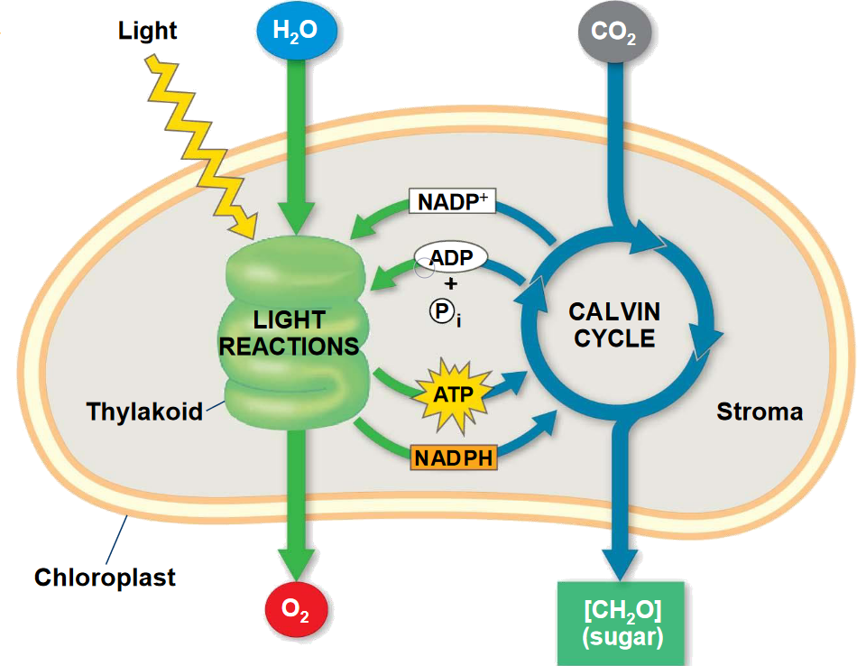
4.3.2 Light reactions
In the reaction centers, the excitation energy of the chlorophyll is used for splitting electrons from water molecules, producing oxygen (O2) as a “side-product”. The electrons are transported along the electron transport chain and are used to produce NADPH and ATP. These are called the light reactions of photosynthesis. Up to here, radiation energy has been converted into chemical energy in the form of ATP. The production of ATP consumes inorganic phosphate.
4.3.3 Calvin cycle
NADPH and ATP are then used for reducing CO2 (the energy-demanding reversal of oxidation) in the Calvin cycle. This step forms C3 compounds (triose-phosphates) and occurs independently of light. It is therefore commonly referred to as the “dark reactions” of photosynthesis. Rubisco (ribulose-1,5-bisphosphate carboxylase/oxygenase) is the principal enzyme involved in the Calvin cycle and the amount of Rubisco determines the capacity for the carboxylation of RuBP (Ribulose-1,5-bisphosphate). Rubisco also catalyzes the oxygenation of RuBP which consumes O2 and produces CO2 as part of photorespiration. This respiration scales with photosynthetic activity and reduces the net photosynthetic CO2 by 30-50%, depending on the relative concentrations of CO2 and O2. At very low CO2 levels, at around 30-50 ppm, the photorespiratory compensation point (\(\Gamma^\ast\)) is reached and net photosynthesis is zero. In contrast to photorespiration, dark respiration (\(R_d\)), which also produces CO2, arises from the decarboxylation of Rubisco and is independent of light, but proportional to the amount of Rubisco.
Reduced C in the form of sucrose or (after an additional step) starch is either consumed in the leaf during the night, or exported through the phloem and used for synthesising biomass or supplying plant-internal C storage as non-structural C (see Chapter 5).
4.3.4 Summary
The chemical summary equation of photosynthesis is: \[ n\mathrm{CO}_2 + 2n\mathrm{H}_2\mathrm{O} \rightarrow (\mathrm{CH}_2\mathrm{O})_n + n\mathrm{O}_2 + n\mathrm{H}_2\mathrm{O} \tag{4.6}\] A total of eight photons is consumed to assimilate one molecule of CO2. For each molecule of CO2, one molecule of O2 is produced. And for each molecule of CO2, one molecule of H2O is consumed (net). Note however, that this water consumption is not the primary reason for why plants use water. A much larger amount of water is consumed by the diffusion of water vapor from the water-saturated air inside the leaves out of the stomata. This transpiration flux is further explained in Chapter 7.
4.3.5 Response to light and CO2
The three steps described above operate in series, and each step is potentially rate-limiting and responds differently to the environment. The rates of the processes are coordinated such that they are roughly equal and co-limiting for average environmental conditions to which a leaf is exposed during a day. An imbalance of rates can lead to an excess production of electrons and can cause damage to the photosynthetic apparatus. This happens, for example, when leaves are exposed to very cold temperatures and high light during a frost event, or when you move your indoor plant that has been sitting in a dark corner for years suddenly into full sunlight outdoors.
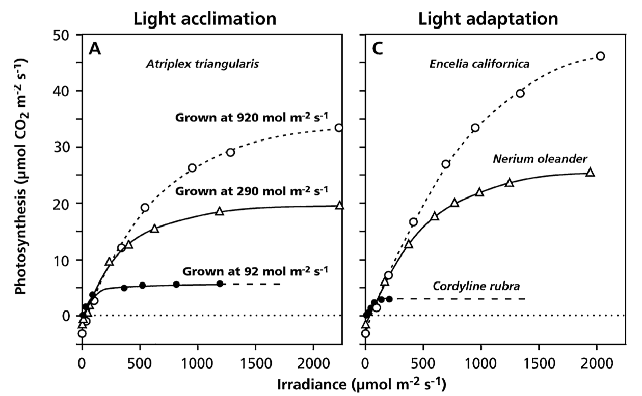
The response of photosynthetic CO2 assimilation (\(A\)) to light (PPFD) and leaf-internal CO2 (\(c_i\)) reflects the serial nature of how the light and dark reactions are connected. \(A\) saturates both in response to increasing PPFD as well as to increasing \(c_i\). When a leaf is exposed to increasing PPFD, \(A\) initially increases and eventually saturates (Figure 4.5). The slope of the initial linear increase reflects the efficiency at which photons are used for CO2 assimilation in the light reactions (the quantum yield \(\varphi_0\)). Under these conditions, light, i.e. the rate of the light reactions, is limiting, not CO2 inside the leaf. Under conditions of very high light, the dark reactions of the Calvin cycle become limiting. The assimilation rate attained under saturating light is commonly referred to as \(A_\mathrm{sat}\).
The level at which the light response of \(A\) saturates (\(A_\mathrm{sat}\)) varies within a species and across different plant species. Variations within species arise through the acclimation of the light reaction capacities to the typical light intensities to which a leaf is exposed. Acclimation of photosynthesis evolves over time scales of weeks to months. (Thus, your indoor plant suffers because the change to high-light conditions happened to fast.) \(A_\mathrm{sat}\) also varies across species, reflecting the adaptation through evolution of different plant species to the environment in which they commonly grow. A typical light adaptation to different light levels is expressed by plants that commonly grow in the shady understorey versus plants that grow in the sun-exposed upper canopy.
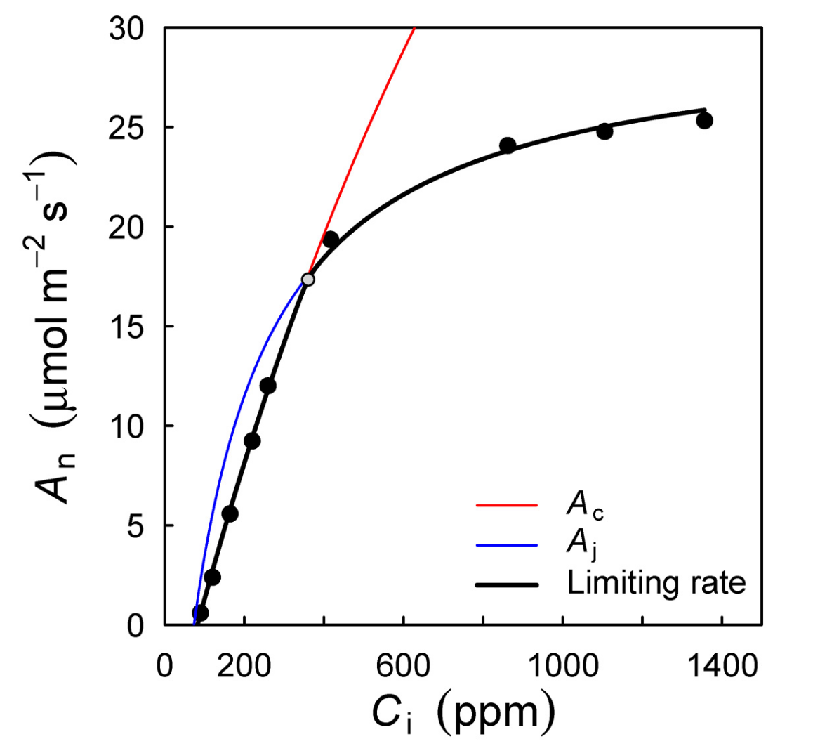
In a similar fashion, the response of \(A\) to \(c_i\) initially increases and saturates at high \(c_i\). This is reflected by the so-called “A-ci curve” (Figure 4.6). Commonly, net assimilation \(A_n = A - R_d\) is considered when analysing A-ci curves. \(A_n\) is initially negative until the photorespiratory compensation point (\(\Gamma^\ast\)) is reached. Then, \(A_n\) increases steeply with \(c_i\) as it is limited by the rate of RuBP carboxylation by Rubisco. This Rubisco carboxylation-limited functional response of assimilation is commonly denoted \(A_C\).
As \(c_i\) increases further, \(A\) is no longer limited by RuBP carboxylation, but by the rate at which RuBP becomes available. This, in turn, is governed by the rate at which ATP and NADPH are produced and thus by the rate of electron transport \(J\). This functional response of assimilation is commonly denoted \(A_J\). A limiting electron transport rate may be due to limiting light or a limiting capacity of electron transport (\(J_\mathrm{max}\)). A slower further increase of \(A\) with \(c_i\) in the electron transport-limited range is due to the suppression of RuBP oxygenation at high concentrations of CO2 (relative to O2). The effective assimilation rate across the full range of \(c_i\) is the minimum of the electron transport-limited and the RuBP carboxylation-limited rate: \[ A_n = \min(A_C, A_J) - R_d \tag{4.7}\]
The A-ci curve (Figure 4.6) can be measured in the field and reveals the rates and efficiencies of the individual processes of the photosynthesis “chain” (light and dark reactions). These quantities are key for quantitatively describing and modeling leaf photosynthesis (see Box Farquhar-von Caemmerer-Berry model below).
NoteFarquhar-von Caemmerer-Berry model
Following the Farquhar-von Caemmerer-Berry (FvCB) model for C3 photosynthesis (Farquhar, Caemmerer, and Berry 1980), the RuBP carboxylation-limited assimilation rate \(A_C\) can be described as \[ A_C = V_\mathrm{cmax} \frac{c_i - \Gamma^\ast}{c_i + K} \;, \tag{4.8}\] where \(K\) is the effective Michaelis-Menten coefficient for \(A_C\), considering the balance of carboxylation and oxygenation by Rubisco. It depends on the partial pressure of oxygen (\(p\mathrm{O}_2\)). \[ K = K_c \left(1 + \frac{p\mathrm{O}_2}{K_o} \right) \] \(V_\mathrm{cmax}\), \(K_c\), \(K_o\), and \(\Gamma^\ast\) all have a temperature dependency. In addition, \(\Gamma^\ast\) is proportional to atmospheric pressure. These dependencies are shown in Section 4.3.6 and are described in full detail in Stocker et al. (2020).
The electron transport-limited assimilation rate \(A_J\) can be described as \[ A_J = \frac{J}{4} \cdot \frac{c_i - \Gamma^\ast}{c_i + 2 \Gamma^\ast}\;. \tag{4.9}\] The electron transport rate \(J\) is described by a saturating function that increases with absorbed light \(I_\mathrm{abs}\) up to a maximum rate \(J_\mathrm{max}\) \[ J = \frac{4\varphi_0 I_\mathrm{abs}}{\sqrt{1+\left(\frac{4\varphi_0 I_\mathrm{abs}}{J_\mathrm{max}}\right)^2}} \tag{4.10}\]
Together, Equation 14.5 and Equation 4.9 describe the combined effect of \(c_i\), (leaf) temperature, the absorbed photon flux density, and atmospheric pressure on leaf-level CO2 assimilation.
With the mathematical description of \(A_C\) and \(A_J\) and their dependency on light and CO2 following the FvCB model, A-ci and the A vs. PPFD curves, as shown for measurements in Figure 4.5 and Figure 4.6, can thereby be modeled.
Code
library(rpmodel)
library(dplyr)
library(tidyr)
library(ggplot2)

# modified seq() function to get a logarithmically spaced sequence
lseq <- function(from=1, to=100000, length.out=6) {
  exp(seq(log(from), log(to), length.out = length.out))
}

# Set model parameters (constants)
# see Stocker et al., 2020 GMD for a description
beta <- 146          # unit cost ratio a/b
c_cost <- 0.41       # marginal cost of Jmax
gamma <- 0.105       # unit cost ratio c/b
kphio <- 0.085       # quantum yield efficiency
c_molmass <- 12.0107 # molar mass, g / mol

# Define environmental conditions
tc <- 15             # temperature, deg C
ppfd <- 500          # micro-mol/m2/s
vpd  <- 300          # Pa
co2  <- 400          # ppm
elv  <- 0            # m.a.s.l.
fapar <- 1           # fraction
patm <- 101325       # Pa

# get photosynthesis parameters gammastar, vcmax, jmax from p-model
# this assumes vcmax and jmax to be optimally acclimated/adapted to
# the specified environmental conditions and considers the temperature
# and atmospheric-pressure dependence of all parameters.
out_pmodel <- rpmodel(
  tc             = tc,
  vpd            = vpd,
  co2            = co2,
  elv            = elv,
  kphio          = kphio,
  beta           = beta,
  fapar          = fapar,
  ppfd           = ppfd,
  method_jmaxlim = "wang17",
  do_ftemp_kphio = FALSE
  )

# electron transport-limited assimilation rate as a function of CO2 partial pressure
calc_aj <- function(ci, gammastar, kphio, ppfd, jmax){
  kphio * ppfd * (ci - gammastar)/(ci + 2 * gammastar) * 1/sqrt(1+((4 * kphio * ppfd)/jmax)^2)
}

# RuBP carboxylation-limited assimilation rate as a function of CO2 partial pressure
calc_ac <- function(ci, gammastar, kmm, vcmax){
  vcmax * (ci - gammastar)/(ci + kmm)
}

# assimilation rate given stomatal conductance and leaf-internal
# CO2 partial pressure
calc_a_gs <- function(ci, gs, ca){
  gs * (ca - ci)
}

# conversion of CO2 concentration in ppm to partial pressure in Pa
co2_to_ca <- function( co2, patm ){
  ( 1.0e-6 ) * co2 * patm
}

df_ci <- tibble(
  ci = seq(0, 1000, length.out = 100)) |>
  rowwise() |>
  mutate(ci_pa = co2_to_ca(ci, patm = patm)) |>
  mutate(a_j = calc_aj(ci_pa,
                       out_pmodel$gammastar,
                       kphio = kphio,
                       ppfd = ppfd,
                       jmax = out_pmodel$jmax)) |>
  mutate(a_c = calc_ac(ci_pa,
                       out_pmodel$gammastar,
                       out_pmodel$kmm,
                       vcmax = out_pmodel$vcmax)) |>
  mutate(a_act = min(a_j, a_c)) |>
  mutate(a_gs = calc_a_gs(ci_pa,
                          gs = out_pmodel$gs,
                          ca = out_pmodel$ca))

df_ci |>
  pivot_longer(cols = c(
    a_j,
    a_c
    # a_gs
    ),
    names_to = "Rate",
    values_to = "a_") |>
  ggplot(aes(x = ci)) +
  geom_line(aes(y = a_, color = Rate)) +
  geom_line(aes(y = a_act)) +
  xlim(00, 1000) +
  # ylim(-20, 80) +
  geom_hline(yintercept = 0, linetype = "dotted") +
  geom_vline(xintercept = 0, linetype = "dotted") +
  geom_vline(xintercept = (out_pmodel$gammastar/(1.0e-6 * patm)), linetype = "dotted") +
  labs(x = expression(paste(italic("c")[i], " (ppm)")),
       y = expression(paste(italic("A"), " (", mu, "mol m" ^{-2}," s" ^{-1}, ")"))) +
  scale_color_manual(
    name = "",
    breaks = c(
      # "a_gs",
      "a_j",
      "a_c"
      ),
    labels = c(
      # expression(paste(italic("A")[gs])),
      expression(paste(italic("A")[J])),
      expression(paste(italic("A")[C]))
      ),
    values = c(
      # "#009E73",
      "#56B4E9",
      "#E69F00"
      )) +
  theme_classic()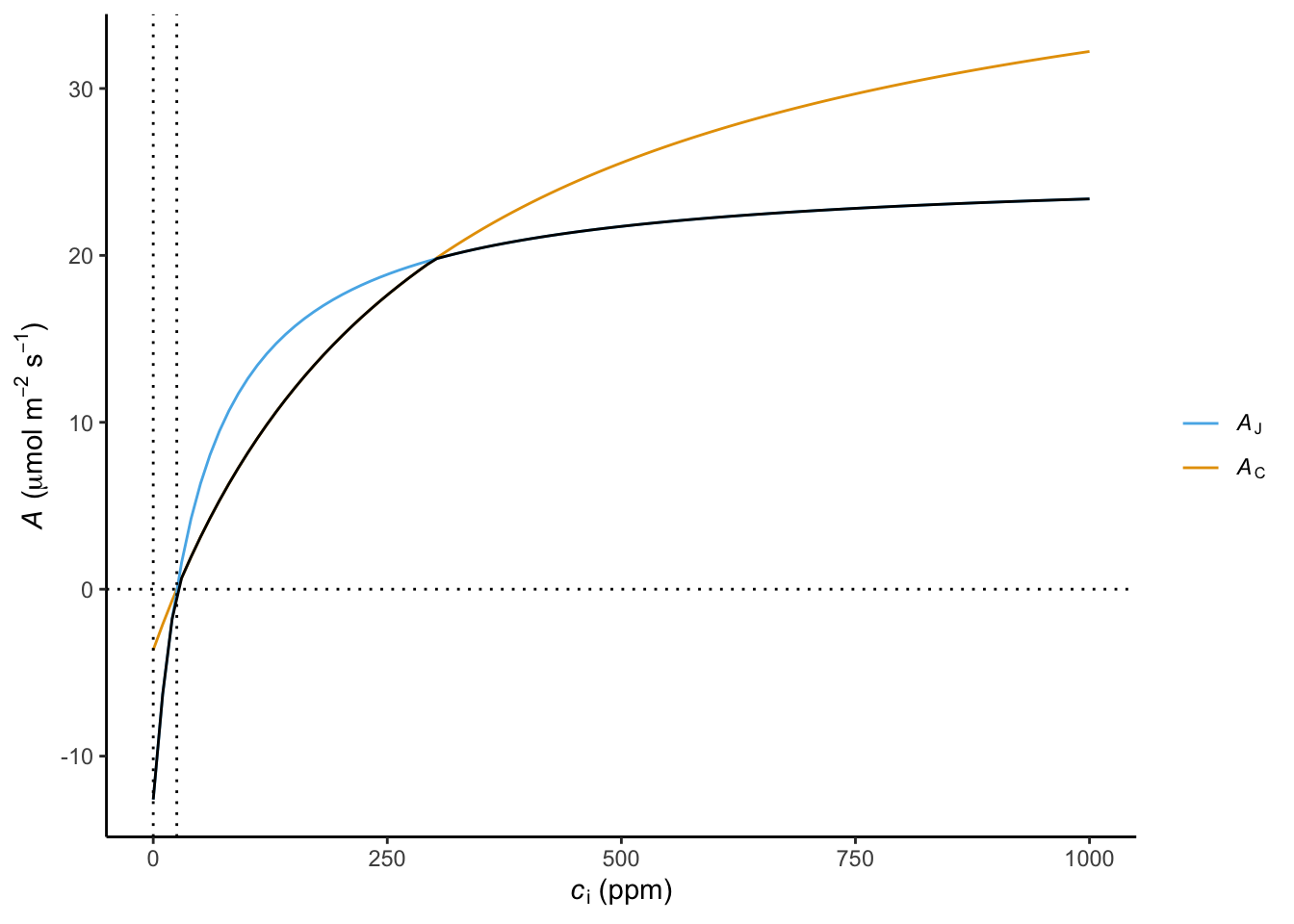
Figure 4.8 shows the light response curve of \(A_J - R_d\) following the FvCB model. The response is shown for leaves acclimated to different levels of light, thus having different values for \(J_\mathrm{max}\). Because acclimation to light also involves a change in the Rubisco content of leaves and thus \(V_\mathrm{cmax}\), “high-light leaves” also have higher dark respiration rates. Therefore, under low light conditions, leaves acclimated to low light have higher net assimilation rates than leaves acclimated to high light. This is illustrated by Figure 4.8 a.
Code
library(rpmodel)
library(dplyr)
library(tidyr)
library(ggplot2)

# modified seq() function to get a logarithmically spaced sequence
lseq <- function(from=1, to=100000, length.out=6) {
  exp(seq(log(from), log(to), length.out = length.out))
}

# Set model parameters (constants)
# see Stocker et al., 2020 GMD for a description
beta <- 146          # unit cost ratio a/b
c_cost <- 0.41       # marginal cost of Jmax
gamma <- 0.105       # unit cost ratio c/b
kphio <- 0.085       # quantum yield efficiency
c_molmass <- 12.0107 # molar mass, g / mol

# Define environmental conditions
tc <- 15             # temperature, deg C
ppfd <- 500          # micro-mol/m2/s
vpd  <- 300          # Pa
co2  <- 400          # ppm
elv  <- 0            # m.a.s.l.
fapar <- 1           # fraction
patm <- 101325       # Pa

# get photosynthesis parameters gammastar, vcmax, jmax from p-model
# this assumes vcmax and jmax to be optimally acclimated/adapted to
# the specified environmental conditions and considers the temperature
# and atmospheric-pressure dependence of all parameters.

# first for low light
out_pmodel_lo <- rpmodel(
  tc             = tc,
  vpd            = vpd,
  co2            = co2,
  elv            = elv,
  kphio          = kphio,
  beta           = beta,
  fapar          = fapar,
  ppfd           = ppfd*0.5,
  method_jmaxlim = "wang17",
  do_ftemp_kphio = FALSE
  )

# medium light
out_pmodel_me <- rpmodel(
  tc             = tc,
  vpd            = vpd,
  co2            = co2,
  elv            = elv,
  kphio          = kphio,
  beta           = beta,
  fapar          = fapar,
  ppfd           = ppfd,
  method_jmaxlim = "wang17",
  do_ftemp_kphio = FALSE
  )

# high light
out_pmodel_hi <- rpmodel(
  tc             = tc,
  vpd            = vpd,
  co2            = co2,
  elv            = elv,
  kphio          = kphio,
  beta           = beta,
  fapar          = fapar,
  ppfd           = ppfd*2,
  method_jmaxlim = "wang17",
  do_ftemp_kphio = FALSE
  )

# electron transport-limited assimilation rate as a function of CO2 partial pressure
calc_aj <- function(ci, gammastar, kphio, ppfd, jmax){
  kphio * ppfd * (ci - gammastar)/(ci + 2 * gammastar) * 1/sqrt(1+((4 * kphio * ppfd)/jmax)^2)
}

# RuBP carboxylation-limited assimilation rate as a function of CO2 partial pressure
calc_ac <- function(ci, gammastar, kmm, vcmax){
  vcmax * (ci - gammastar)/(ci + kmm)
}

# assimilation rate given stomatal conductance and leaf-internal
# CO2 partial pressure
calc_a_gs <- function(ci, gs, ca){
  gs * (ca - ci)
}

# conversion of CO2 concentration in ppm to partial pressure in Pa
co2_to_ca <- function( co2, patm ){
  ( 1.0e-6 ) * co2 * patm
}

df_ppfd <- tibble(
  ppfd = seq(0, 2000, length.out = 100)) |>
  rowwise() |>
  mutate(a_j_lo = calc_aj(co2_to_ca(400, patm = patm),
                          out_pmodel_lo$gammastar,
                          kphio = kphio,
                          ppfd = ppfd,
                          jmax = out_pmodel_lo$jmax * 0.5) -
           out_pmodel_lo$rd) |>
  mutate(a_j_me = calc_aj(co2_to_ca(400, patm = patm),
                       out_pmodel_me$gammastar,
                       kphio = kphio,
                       ppfd = ppfd,
                       jmax = out_pmodel_me$jmax) -
           out_pmodel_me$rd) |>
  mutate(a_j_hi = calc_aj(co2_to_ca(400, patm = patm),
                          out_pmodel_hi$gammastar,
                          kphio = kphio,
                          ppfd = ppfd,
                          jmax = out_pmodel_hi$jmax * 2) -
           out_pmodel_hi$rd)

gg <- df_ppfd |>
  pivot_longer(cols = c(a_j_lo, a_j_me, a_j_hi),
               names_to = "Rate",
               values_to = "a_") |>
  ggplot(aes(x = ppfd)) +
  geom_line(aes(y = a_, color = Rate)) +
  geom_hline(yintercept = 0, linetype = "dotted") +
  labs(x = expression(paste("PPFD (", mu, "mol m"^{-2}, "s"^{-1}, ")")),
       y = expression(paste(italic("A")[J] - italic(R)[d], " (", mu, "mol m" ^{-2}," s" ^{-1}, ")"))) +
  scale_color_manual(
    name = "",
    breaks = c("a_j_lo",
               "a_j_me",
               "a_j_hi"
               ),
    labels = c(expression(paste("Low light")),
               expression(paste("Medium light")),
               expression(paste("High light"))),
    values = c( "#009E73", "#56B4E9", "#E69F00")) +
  theme_classic()

gg1 <- gg +
  xlim(0, 250) +
  ylim(NA, 20)

gg2 <- gg +
  xlim(0, 2000)

cowplot::plot_grid(gg1, gg2,
                   nrow = 2,
                   labels = c("a", "b"))
Note that the FvCB model, on its own, does not allow us to model the LUE term in Equation 4.1. An important additional ingredient is the stomatal conductance (\(g_s\)) which is relevant for determining the ratio of ambient to leaf-internal CO2 concentrations. It is described in Section 4.4.
4.3.6 Response to temperature
All processes involved in photosynthesis are strongly affected by temperature. Enzymatic rates, like Rubisco carboxylation, have a temperature at which reaction rates have a maximum. As a consequence, assimilation rates also attain a maximum at a certain temperature–the temperature optimum (Topt). In contrast, dark respiration (\(R_d\)) monotonically increases with temperature. That is, it continues to rise as temperatures go up without attaining a maximum. As a consequence, the decline of net assimilation rates is even faster towards high temperatures than that of gross assimilation rates.
The temperature dependency of leaf CO2 assimilation rates can be measured in the field by exposing a leaf to a range of temperatures (within a relatively short period of time) and measuring assimilation rates for each temperature. When looking at such measurements, a temperature optimum of net photosynthesis is evident.
The Farquhar-von Caemmerer Berry model for C3 photosynthesis (see Box ‘Farquhar von Caemmerer Berry model’) and the mathematical description of temperature dependencies of factors therein (\(V_\mathrm{cmax}\), \(J_\mathrm{max}\), \(K_c\), \(K_o\), and \(\Gamma^\ast\), temperature dependencies not shown here) provide a basis for modelling the temperature dependency of assimilation rates. Such modelled temperature dependencies are shown in Figure 4.9.
Code
df_temp <- tibble(
  temp = seq(0, 40, length.out = 100)) |>
  rowwise() |>
  mutate(gammastar = calc_gammastar(temp, patm = 101325),
         kmm = calc_kmm(temp, patm = 101325),
         vcmax = out_pmodel$vcmax25 * ftemp_inst_vcmax(temp, tcgrowth = 15),
         jmax = 1.7 * out_pmodel$vcmax25 * ftemp_inst_jmax(temp, tcgrowth = 15),
         rd = 0.05 * out_pmodel$vcmax25 * ftemp_inst_rd(temp)
         ) |>
  mutate(a_j = calc_aj(ci = 28.14209,
                       gammastar,
                       kphio = kphio,
                       ppfd = ppfd,
                       jmax = jmax)) |>
  mutate(a_c = calc_ac(ci = 28.14209,
                       gammastar,
                       kmm,
                       vcmax = vcmax)) |>
  mutate(a_cr = a_c - rd,
         a_jr = a_j - rd) |>
  mutate(assim = min(a_jr, a_cr))

gg1 <- df_temp |>
  pivot_longer(cols = c(gammastar, kmm),
               names_to = "Rate",
               values_to = "value") |>
  ggplot(aes(x = temp)) +
  geom_line(aes(y = value, color = Rate)) +
  geom_hline(yintercept = 0, linetype = "dotted") +
  labs(x = expression(paste("Temperature (°C)")),
       y = expression(paste("Value (Pa)"))) +
  khroma::scale_color_okabeito(
    name = "",
    breaks = c("gammastar",
               "kmm"),
    labels = c(expression(paste(italic(Gamma)^"*")),
               expression(italic(K)))
    ) +
  theme_classic()

gg2 <- df_temp |>
  pivot_longer(cols = c(vcmax, jmax, rd),
               names_to = "Rate",
               values_to = "value") |>
  ggplot(aes(x = temp)) +
  geom_line(aes(y = value, color = Rate)) +
  geom_hline(yintercept = 0, linetype = "dotted") +
  labs(x = expression(paste("Temperature (°C)")),
       y = expression(paste("Rate (", mu, "mol m" ^{-2}," s" ^{-1}, ")"))) +
  khroma::scale_color_okabeito(
    name = "",
    breaks = c("vcmax",
               "jmax",
               "rd"),
    labels = c(expression(paste(italic("V")[cmax])),
               expression(paste(italic("J")[max])),
               expression(paste(italic("R")[d])))
    ) +
  theme_classic()

df_net_plot <- df_temp |>
  mutate(a_cr = a_c - rd,
         a_jr = a_j - rd) |>
  pivot_longer(cols = c(rd, a_cr, a_jr, assim),
               names_to = "Rate",
               values_to = "value")

df_gross_plot <- df_temp |>
  pivot_longer(cols = c(a_c, a_j),
               names_to = "Rate",
               values_to = "value")

gg3 <- ggplot() +
  geom_line(aes(x = temp, y = value, color = Rate),
            data = df_gross_plot,
            linetype = "dashed") +
  geom_line(aes(x = temp, y = value, color = Rate),
            data = df_net_plot) +
  geom_hline(yintercept = 0, linetype = "dotted") +
  scale_color_manual(
    name = "",
    breaks = c("rd",
               "a_c",
               "a_j",
               "a_cr",
               "a_jr",
               "assim"
               ),
    labels = c(expression(paste(italic("R")[d])),
               expression(paste(italic("A")[C])),
               expression(paste(italic("A")[J])),
               expression(paste(italic("A")[C] ~ - ~ italic("R")[d])),
               expression(paste(italic("A")[J] ~ - ~ italic("R")[d])),
               expression(paste(italic("A")[n]))),
    values = c("#CC79A7", "#E69F00", "#56B4E9", "#E69F00", "#56B4E9", "black")
  ) +
  labs(x = expression(paste("Temperature (°C)")),
       y = expression(paste(italic("A"), "(", mu, "mol m" ^{-2}," s" ^{-1}, ")")),
       color = "Rate",
       linetype = "Rate") +
  theme_classic()

cowplot::plot_grid(gg1, gg2, gg3, ncol = 1)
Ignoring unknown labels:
• linetype : "Rate"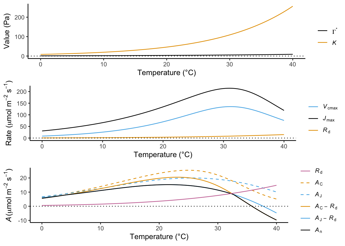
4.3.7 Adaptation and acclimation of Topt
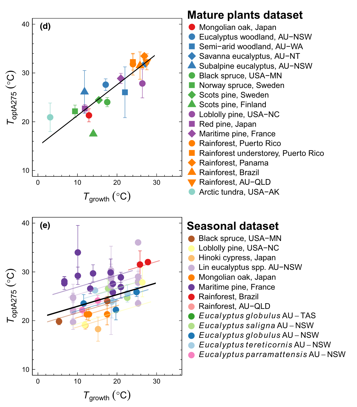
The temperature dependencies shown in Figure 4.9 are instantaneous responses. That is, they represent the responses to changes in temperature that evolve over short time scales–minutes to hours. Over longer time scales, the shapes of the instantaneous temperature responses change. The temperature optimum of photosynthesis (Topt) tends to be higher for plant species that grow in warm climates than for plants that can be found in cold climates (Figure 4.10 a). Such variations of Topt across different plant species reflect species’ adaptation to their growth environment which makes them perform well and compete effectively under certain environmental conditions and is related to their genes and is thus passed on from generation to generation. Topt can be considered as a plant trait (see Section 2.4).
Topt not only varies between species growing in different climates, but can also vary within a given species and even within a given plant when it is exposed to different temperatures for a longer period (Kumarathunge et al. 2019). Given enough time, the instantaneous temperature response and Topt will shift to higher temperatures as a result of persistent exposure to warmer temperatures. Such variations in a plant trait (here Topt) within species and an individual plant is referred to as acclimation. Figure 4.10 b shows how Topt varies within different species (distinguished by color) over the course of the seasons - a demonstration of acclimation.
Acclimation is relatively common to observe also for other physiological traits than Topt. For example, photosynthetic capacities (the maximum rate of Rubisco carboxylation - \(V_\mathrm{cmax}\) in the FvCB model - or the maximum rate of electron transport - \(J_\mathrm{max}\)) acclimate over the course of seasons (Jiang et al. 2020). Other plant traits are less plastic or not plastic at all. For example, phenological strategies (e.g., deciduousness) do not acclimate. The acclimation of physiological traits is important for understanding vegetation and land carbon cycle responses to long-term trends in climate. While it may be expected that plants have a certain capacity for acclimation to a new climate, limits to acclimation must be better understood.
4.3.8 C4 photosynthesis
Coming soon.
4.4 Transpiration and leaf water-carbon coupling
The opening of stomata is highly sensitive to environmental factors, and the CO2 assimilation rate feeds back to stomatal opening. By opening and closing stomata, plants regulate the conductance to CO2 diffusion from the ambient air into the leaves and to the photosynthesis reaction sites. Simultaneously, when stomata are open, water vapor diffuses out of the leaf - transpiration. This link between CO2 and water loss is at the core of stomatal regulation to balance C uptake and desiccation.
The diffusive supply of CO2 to the photosynthetic reaction sites is determined by a series of conductances. The description of the diffusive CO2 uptake in Equation 4.5 resolves this as a single conductance. However, stomatal conductance is only one chain in this series. More realistically, the leaf boundary layer conductance and the mesophyll conductance are treated separately from the stomatal conductance. However, because the leaf boundary layer conductance is much larger than the stomatal conductance, it is not limiting. Furthermore, actively regulated plant physiological responses to the environment arise through the stomatal conductance \(g_s\). As described in Section 4.3, mesophyll conductance is often ignored due to practical limitations for separating it from stomatal conductance in measurements and due to very poorly known dependencies to the environment. Hence, we focus on \(g_s\) here and describe the diffusive CO2 supply to photosynthesis by Equation 4.5.
The diffusive water vapor flux out of the leaf - transpiration - is driven by the difference of water vapor pressure in the leaf-interior air spaces (\(e_i\)) and the the water vapor pressure at the leaf surface (\(e_s\)). Their difference is commonly referred to as the vapor pressure deficit (VPD), here denoted as \(D = e_s - e_i\). Leaf-interior air spaces are water vapor-saturated, while the surrounding air is not. Fick’s law predicts that a diffusive flux occurs in presence of a concentration difference, hence transpiration can be described as \[ E = 1.6 \; g_s \; D \tag{4.11}\] The factor 1.6 arises due to the lower diffusivity of CO2 compared with H2O. Hence, \(g_s\) has to be understood as a conductance to CO2 diffusion (mol CO2 m-2 s-1). Note that \(g_s\) regulates both transpiration (Equation 4.11) and assimilation (Equation 4.5) at the leaf-level. A tight coupling between water and carbon fluxes at the leaf-level follows from the physical principle of diffusion.
Water loss through transpiration poses risks and incurs costs for a plant. The diffusive water vapor flux through stomata has to be maintained by root water uptake from the soil and transport along the xylem in the plant. When the water content in the rooting zone declines, it becomes increasingly hard for plants to extract water from the soil and they have to “suck” out the water with a increasingly negative water potential–a negative pressure. The hydraulic relationships of water transport along the soil-plant-atmosphere continuum will be introduced later. What matters here is that such negative water potentials along the water transport pathway are dangerous for the plant and can lead to lethal desiccation of cells, leaves, branches, or entire plants.
Avoidance of dangerous desiccation is enabled by responses at the level of leaves and the plant which operate at a range of time scales. At time scales of seconds to minutes and at the level of a leaf, stomatal conductance is reduced in response to dry air and dry soil conditions. At time scales of weeks to months, or even years, the leaf area of a plant may decline under dry conditions. At even longer time scales (albeit this time scale is subject to large unknowns and active research), plants are genetically adapted (or may acclimate within their lifetime) to dry conditions by resistant water transport (resistant xylem) and effective water uptake organs (deeper roots).
Obviously, such adaptations and the largely instantaneous stomatal response incurs a cost. This may be conceived as an opportunity cost of reduced CO2 assimilation when stomatal conductance is reduced and the construction cost of building water-stress adapted organs. Hence, plants always have to balance carbon uptake and water loss and a tight carbon-water coupling at the level of plants, and ecosystems arises from these leaf-level processes.
4.4.1 Water use efficiency
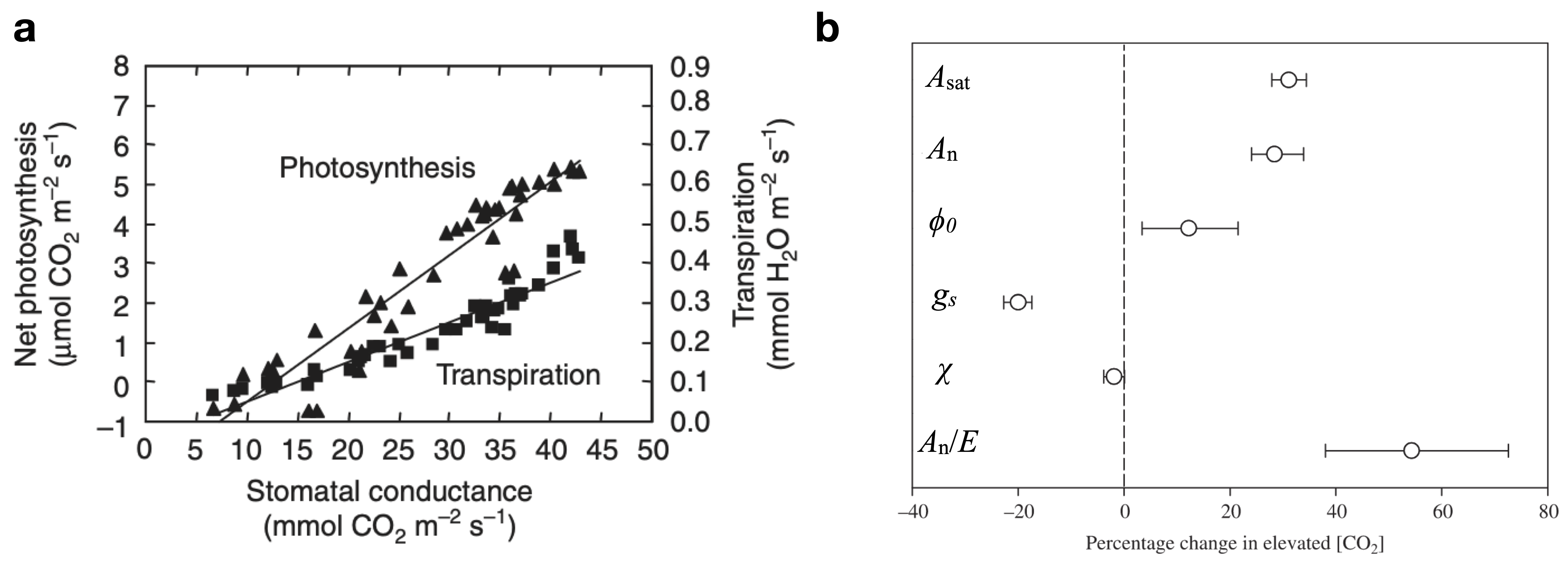
The trade-off between transpiration and assimilation can be measured by considering their ratio by combining Equation 4.5 and Equation 4.11 to define the instantaneous water-use efficiency: \[ \frac{A_n}{E} = \frac{c_a(1 - \chi)}{1.6\;D}\;, \tag{4.12}\] where \(\chi = c_i/c_a\). The instantaneous water-use efficiency is proportional to \(D^{-1}\). In other words, the drier the air, the more transpiration per unit net CO2 assimilation a leaf “suffers”. This demonstrates the strong effect of atmospheric dryness on the water-carbon trade-off. To remove the effect of vapor pressure deficit (\(D\)) on transpiration and focus on the biological component of the water-carbon trade-off, the intrinsic water-use efficiency (iWUE) is defined by relating net assimilation to stomatal conductance: \[ \frac{A_n}{g_s} = \frac{c_a}{1.6}(1 - \chi) \tag{4.13}\] Note that Equation 4.12 and Equation 4.13 are written as being proportional to \(c_a(1-\chi)\). Of course, this term is mathematically equivalent to \((c_a - c_i)\). However, there is a reason for expressing it this way. First, it reflects the direct influence of \(c_a\) ambient (atmospheric) CO2 concentration on the water-carbon trade-off - less water is lost for a given amount of C assimilation under elevated CO2. Second, observations suggest that \(\chi\) is regulated by plants to remain relatively constant under a wide range of CO2 levels (Ainsworth and Long 2005) and Figure 4.11. The near constancy of \(\chi\) is also reflected by the observation that \(A_n\) and \(g_s\) vary in near proportion across a wide range of light levels (Bonan 2015).
4.4.2 Isotopic fractionation
Coming soon.
4.4.3 Stomatal regulation
The closing of stomates and the reduction of stomatal conductance \(g_s\) under dry conditions prevents plants from dangerous desiccation. However, a reduced \(g_s\) also leads to a reduction in CO2 diffusion into leaves and thus a reduction of photosynthetic CO2 assimilation. Hence, plants have to balance a trade-off between carbon gain and the risk of desiccation. A complete stomatal closure under moderately dry conditions (low soil moisture, high VPD) may be safe in terms of desiccation avoidance but comes at an excessive cost in terms of foregone CO2 uptake (and similarly vice-versa). An optimal strategy must lie somewhere in between these extreme strategies.
Observations of leaf and ecosystem fluxes CO2 and water vapor fluxes document how stomatal conductance responds to increasing VPD and decreasing soil moisture. Figure 4.12 shows this for measurements taken at the ecosystem-level, quantifying the canopy stomatal conductance (denoted by an uppercase \(G_s\)), representative for the collective behaviour of all leaves in the canopy. Three important aspects of this relationship stand out. First, \(G_s\) declines in response to VPD in a non-linear fashion (high sensitivity to VPD at low VPD, lower sensitivity towards higher VPD). Second, there is an interaction between the effect of VPD and soil moisture. Under conditions of dry soils, \(G_s\) is reduced compared to wet soils, given the same VPD. Third, at the moistest site (Figure 4.12 a), \(G_s\) under moist conditions (moist soils, low VPD) is highest but declines most rapidly with VPD.

A simple empirical model for the \(G_s\) response to VPD (Oren et al. 2001) is given by \[ G_s = G_{s,\mathrm{ref}} \left(1 - m \ln D \right)\;. \] Here, \(G_{s,\mathrm{ref}}\) is a reference canopy conductance, \(D\) is VPD, and \(m\) is a stomatal sensitivity parameter. The data shown in Figure 4.12 indicate that the sensitivity parameter \(m\) is not a constant, but decreases with drying soils and tends to be lower at dry sites than at moist sites investigated by Novick et al. (2016).
TipStomatal optimization models
The aspect that plants regulate stomatal conductance to balance the trade-off between carbon gain and water loss lends itself to modelling the stomatal response considering optimality principles. Indeed, there is empirical evidence that optimality models are a good representation of how stomata are regulated. Following this notion, it can be assumed that stomatal conductance is optimised such that the net between the carbon gain by increasing stomatal conductance and the carbon cost by the resulting increased transpiration is maximized.
\[ A - aE - bV_\mathrm{cmax} = \arg \max \tag{4.14}\]
Over time scales of days to weeks, \(V_\mathrm{cmax}\) in the FvCB model (see box above) is coordinated with stomatal conductance (Joshi et al. 2022). The simultaneous effects of \(V_\mathrm{cmax}\) and \(g_s\) are reflected by \(\chi\). Therefore, Equation 4.14 can be expressed with respect to optimising \(\chi\). Maximising a function is equivalent to finding the point where its first derivative (here with respect to \(\chi\)) is zero. (Prentice et al. 2014) formulated such a similar (but not strictly equivalent) optimality criterion as \[ \frac{\partial (E/A)}{\partial \chi} + \beta \frac{\partial (V_\mathrm{cmax}/A)}{\partial \chi} = 0 \;. \] \(E/A\) is the unit cost of transpiration. \(V_\mathrm{cmax}/A\) is the unit cost of carboxylation. Their sum is minimized here with respect to \(\chi\). \(\beta\) is the unit cost ratio. From this, the response of the stomatal conductance to \(D\) and \(A\) can be derived (not shown here, but in Stocker et al. (2020)) as \[ g_s = \left( 1 + \frac{g_1}{\sqrt{D}} \right) \frac{A}{c_a - \Gamma^\ast} \] \(g_1\) is a stomatal sensitivity parameter. Similar results are obtained with a related but not identical optimality criterion (Medlyn et al. 2011).
4.5 From photosynthesis to light use efficiency
The light use efficiency model (Equation 4.1) and the FvCB model (Equation 4.9 and Equation 4.10) represent a contrasting response of photosynthesis to light - linear in Equation 4.1 and saturating (by effects of a finite \(J_\mathrm{max}\)) in Equation 4.9 and Equation 4.10. It should be noted that the LUE model describes the photosynthetic CO2 uptake at the canopy-level and for periods of multiple days to weeks (total GPP vs. total absorbed light). In contrast, the FvCB model describes the light-photosynthesis relationship at the leaf-level and in response to rapid changes in light (e.g., over the course of a day).
As pointed out in Section 4.3.5, plants tend to coordinate the light and carboxylation-limited assimilation rates flexibly in response to average environmental conditions to which they are exposed while performing photosynthesis. Tending towards the co-limitation point can also be understood as an optimal functioning - avoiding overinvestment into maintaining a high maximum electron transport rate (\(J_\mathrm{max}\)) while being carboxylation-limited (too low \(V_\mathrm{cmax}\)), or the opposite. In other words, the higher the average light levels, the higher the maximum carboxylation capacity and therefore the amount of Rubisco in leaves. The linear relationship between GPP and PPFD in Equation 4.1 can be interpreted as an emerging relationship from the coordination of \(A_C\) and \(A_J\), and thus of \(V_\mathrm{cmax}\) and \(J_\mathrm{max}\).
A very simple model, by which LUE is assumed to be constant over time and across ecosystems and using Equation 4.1 explains about 80% of observed GPP variations in data obtained from ecosystem flux measurements, as shown in Figure 4.13. In other words, variations in light (PPFD) and leaf area (measured by fAPAR) explain 80% of GPP variations over the seasons and across different locations on the globe.
Code
library(ggplot2)
library(cowplot)
library(dplyr)
library(tidyr)
library(hexbin)

wdf <- readRDS(here::here("data/wdf_fdk.rds"))

# get absorbed photosynthetically active radiation APAR
wdf <- wdf |>
  mutate(apar = fapar * ppfd)

# fit linear model of GPP ~ APAR with zero intercept
linmod <- lm(gpp ~ 0 + apar, data = wdf)

rsq_val <- summary(linmod)$r.squared
rsq_lab <- format( rsq_val, digits = 2 )

wdf |>
  ggplot(aes(apar, gpp)) +
  # geom_point(alpha = 0.3) +
  geom_hex(bins = 50) +
  scale_fill_viridis_c(trans = "log", option = "magma", name = "Count") +
  geom_abline(intercept = 0, slope = coef(linmod), linetype="dotted") +
  theme_classic() +
  labs(
    x = expression(paste("PPFD"  %*% "fAPAR (mol m"^{-2}, "s"^{-1}, ")")),
    y = expression(paste("GPP (gC m"^{-2}, "s"^{-1}, ")")),
    subtitle = bquote(
        italic(R)^2 == .(rsq_lab)
      ),
    name = ""
  )
CautionExercise
Rising CO2 increases leaf-level photosynthesis. This sensitivity can be quantified using \(\beta\) following Equation 3.8. Calculate \(\beta\) for the light-saturated photosynthesis rate (taking the equation for \(A_C\)), considering an increase in atmospheric CO2 from 400 to 600 ppm. Use \(\Gamma^\ast = 3.3\) Pa, \(K = 46\) Pa and \(V_\mathrm{cmax} = 49 \; \mu\)mol m-2 s-1. Note that \(c_a\) in Equation 4.5 is expressed in Pa. Convert an atmospheric CO2 concentration in units of ppm to Pa by multiplication with 0.101325 Pa ppm-1 (considering standard atmospheric pressure). Assume that the ratio of ambient-to-leaf-internal CO2 (\(\chi\)) remains constant at 0.7.
Compare your calculated \(\beta\) of the light-saturated leaf-level photosynthesis rate with observations from Free Air CO2 Enrichment (FACE) experiments, as summarized by Ainsworth and Long (2005). For this, download the paper here and find the reported value for the CO2 response of the light-saturated leaf-level photosynthesis rate. Convert the percentage increase reported by Ainsworth and Long (2005) into a \(\beta\) factor. Assume that on average, the CO2 levels in the FACE experiments were 350 ppm at ambient and 550 ppm at elevated levels.