
6 Spatial and temporal patterns of the terrestrial carbon cycle
Up to this point, we have considered the global terrestrial C cycle either as a 1-box model in Chapter 4, or as a cascade of boxes in Chapter 5. We have also learned in Chapter 4 and Chapter 5 how the CO2 assimilation and respiration fluxes depend on climatic variables. This implies the fluxes and pools of the terrestrial carbon cycle vary over the course of seasons and days and across geographical space, that is across with different background climates and biomes. In this chapter, we delve into these spatial and temporal patterns of the land carbon cycle.
In Chapter 4, the ecosystem-level photosynthetic CO2 assimilation flux, GPP, was described as a linear function of solar radiation (measured by PPFD), modified by the light use efficiency (LUE) and the fraction of absorbed photosynthetically active radiation (fAPAR). In Section 4.5, we found that such a linear relationship (assuming a temporally constant and spatially uniform LUE) explains around 75% of the variations in GPP across sites and over time (aggregated data to weeks) in the dataset. Since GPP is the ultimate “engine” of the C cycle in terrestrial ecosystems and supplies C for all “downstream” fluxes and pools along the C cascade (Section 5.2), solar radiation is a major control of the terrestrial carbon cycle.
After having introduced how photosynthesis and light use efficiency (LUE) are driven by climate, this chapter introduces the spatial and temporal variations of the other two factors of the LUE model: PPFD and fAPAR. Section 6.1 explains how variations in PPFD received at the top of the canopy at a specific day-of-year and latitude depends on the geometry of how the Earth rotates around the sun. Section 6.2 introduces patterns and simple models for how phenology of vegetation greenness, and therefore fAPAR, evolve. This focuses on leaf unfolding and shedding, with a focus on winter-dormant temperate and boreal biomes. Water stress-driven vegetation greenness changes will be introduced later. Section 6.3 integrates the introduction of the processes into a description of the emerging patterns of GPP across space and time, while Section 6.4 will introduce how ecosystem fluxes and carbon pools vary spatially across the globe.
6.1 Solar radiation
PPFD is a fraction of the solar radiation at the top of the atmosphere (\(I_\mathrm{TOA}\)). This fraction depends on the planetary albedo for visible light (\(\alpha_v\), unitless), an atmospheric attenuation factor (\(\tau\), unitless) that accounts for the elevation (\(z\))-dependent path length of a light ray travelling through the atmosphere and a factor that accounts for cloud cover \(f_c\). A further reduction by about 50% arises because photosynthesis uses only a range of the spectrum of wavelengths of solar radiation, corresponding to the visible light spectrum. The factor \(f_{p}\) accounts for this and for the conversion of \(I_\mathrm{TOA}\), expressed as an energy flux in W m-2, to a flux of photons in mol s-1 m-2. \[ \mathrm{PPFD} = (1-\alpha_{v})\; \tau(z, f_c) \; f_{p} \; I_\mathrm{TOA} \tag{6.1}\]
Equation 6.1 is expressed in units of photon flux. The corresponding relation, expressed in energy units (more common in climatology) is very similar. Solar radiation across the full short-wave spectrum emitted by the sun and incident at the land surface (top-of-canopy, \(I_\mathrm{0}\)) is similarly related to \(I_\mathrm{TOA}\). A different albedo applies for total short-wave radiation vs. the radiation in the photosynthetically active (and visible) spectrum. The factor \(f_{p}\) does not apply here, and \(I_\mathrm{0}\) is commonly expressed in energy units (W m-2). \[ I_\mathrm{0} = (1-\alpha_\mathrm{sw})\; \tau(z, f_c) \; I_\mathrm{TOA} \tag{6.2}\]
6.1.1 Solar geometry
Let’s first step outside the atmosphere and focus on the solar geometry to understand \(I_\mathrm{TOA}\). Solar geometry describes the cyclical movement of the Earth around the sun and how the resulting cyclically varying amount of solar energy that reaches the Earth. The top-of-the atmosphere perspective is relevant to separate atmospheric effects from planetary effects.
\(I_\mathrm{TOA}\) scales in proportion to the solar constant \(I_S\) (1360.8 W m-2) and is inversely proportional to the square of the distance between the Earth and the sun (\(r_E\)). \[ I_\mathrm{TOA} = I_S r_E^{-2} \cos \theta_z \tag{6.3}\] \(\theta_z\) is the solar zenith angle. The term \(\cos \theta_z\) accounts for the dependence of the solar radiation on the angle at which the sun’s rays reach the Earth surface (no terrain considered). It varies cyclically over the course of a day (with hour-of-day) and over the course of a year (with day-of-year). The zenith angle is zero when the sun is directly above the observer - in the zenith (Figure 6.2). At this point, the intensity of the solar radiation is at its maximum.
Note that \(r_E\) is not constant over the course of a year as the Earth rotates around the sun not following a perfect circle but an ellipse.

The dependence of the solar zenith angle on the hour-of-day, day-of-year, and the latitude is described by \[ \cos \theta_z = \sin \varphi \sin \delta +\cos \varphi \cos \delta \cos h \tag{6.4}\]
- \(\varphi\) is the local latitude in radians (0 at the equator, \(\pi/2\) at the poles)
- \(\delta\) is the solar declination angle. It accounts for the tilt of the Earth relative to the plane in which it moves around the sun. It varies with the day-of-year (\(23.5^\circ \pi/180\) on the northern-hemispheric summer solstice, June 21, and \(-23.5^\circ \pi/180\) on the northern-hemispheric winter solstice, December 21)
- \(h\) is the solar hour angle. It varies with the hour-of-day (0 at solar noon, \(\pi\) at “solar midnight”, \(\pi/12\) at 1 hour after solar noon).
A derivation of Equation 6.4 is given on Wikipedia.
6.1.2 Sloped surfaces
Coming soon.
6.1.3 Variations in solar radiation
Variations in the solar zenith angle, as expressed through Equation 6.4, are shown for different latitudes and a mid-summer diurnal cycle in Figure 6.3.
Code
library(ggplot2)
library(cowplot)
library(dplyr)
library(tidyr)

calc_cos_zenith_angle <- function(
    lat, # latitude in degrees
    doy, # day of year (1-365)
    hod  # hour of day (0-24, 12 is solar noon)
){
  doy_summer_solstice <- 173 # day-of-year of summer solstice (21 Jun)
  decl <- 23.5 * cos((doy - doy_summer_solstice) / 365 * 2 * pi) * pi/180
  phi <- lat * pi / 180 # latitude in radians
  hour_angle <- (hod - 12) / 24 * 2 * pi
  cos_zenith_angle <- sin(phi) * sin(decl) + cos(phi) * cos(decl) * cos(hour_angle)

  # limit to zero - sun disappears behind the horizon
  cos_zenith_angle <- ifelse(cos_zenith_angle < 0, 0, cos_zenith_angle)
  return(cos_zenith_angle)
}

# Solar azimuth -------
# at NH summer solstice (doy = 173)
ggplot() +
  # at equator
  geom_function(
    aes(color = "Equator"),
    fun = calc_cos_zenith_angle,
    args = list(
      lat = 0,
      doy = 173
    )) +
  # at tropic (lat = 23.5)
  geom_function(
    aes(color = "23.5° N"),
    fun = calc_cos_zenith_angle,
    args = list(
      lat = 23.5,
      doy = 173
    )) +
  # at polar (lat = 66.5)
  geom_function(
    aes(color = "66.5° N"),
    fun = calc_cos_zenith_angle,
    args = list(
      lat = 66.5,
      doy = 173
    )) +
  # at north pole
  geom_function(
    aes(color = "North pole"),
    fun = calc_cos_zenith_angle,
    args = list(
      lat = 90,
      doy = 173
    )) +
  xlim(0, 24) +
  geom_vline(xintercept = 12, linetype = "dotted") +
  scale_color_viridis_d(
    breaks = c("Equator", "23.5° N", "66.5° N", "North pole"),
    name = ""
  ) +
  labs(title = "Cosine of solar zenith angle",
       subtitle = "Summer solstice (21 June)",
       x = "Hour of day",
       y = "") +
  theme_classic()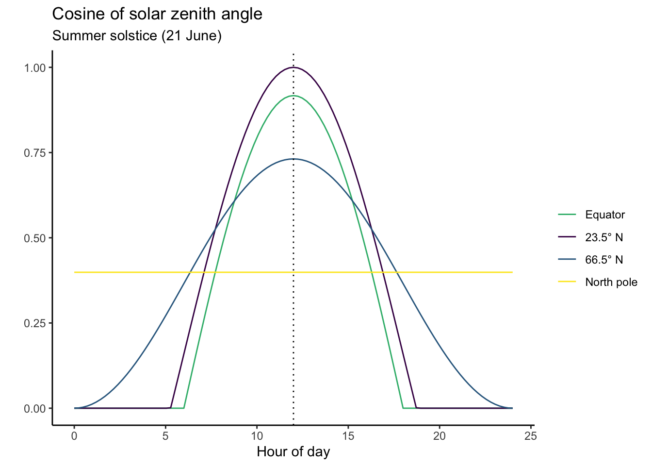
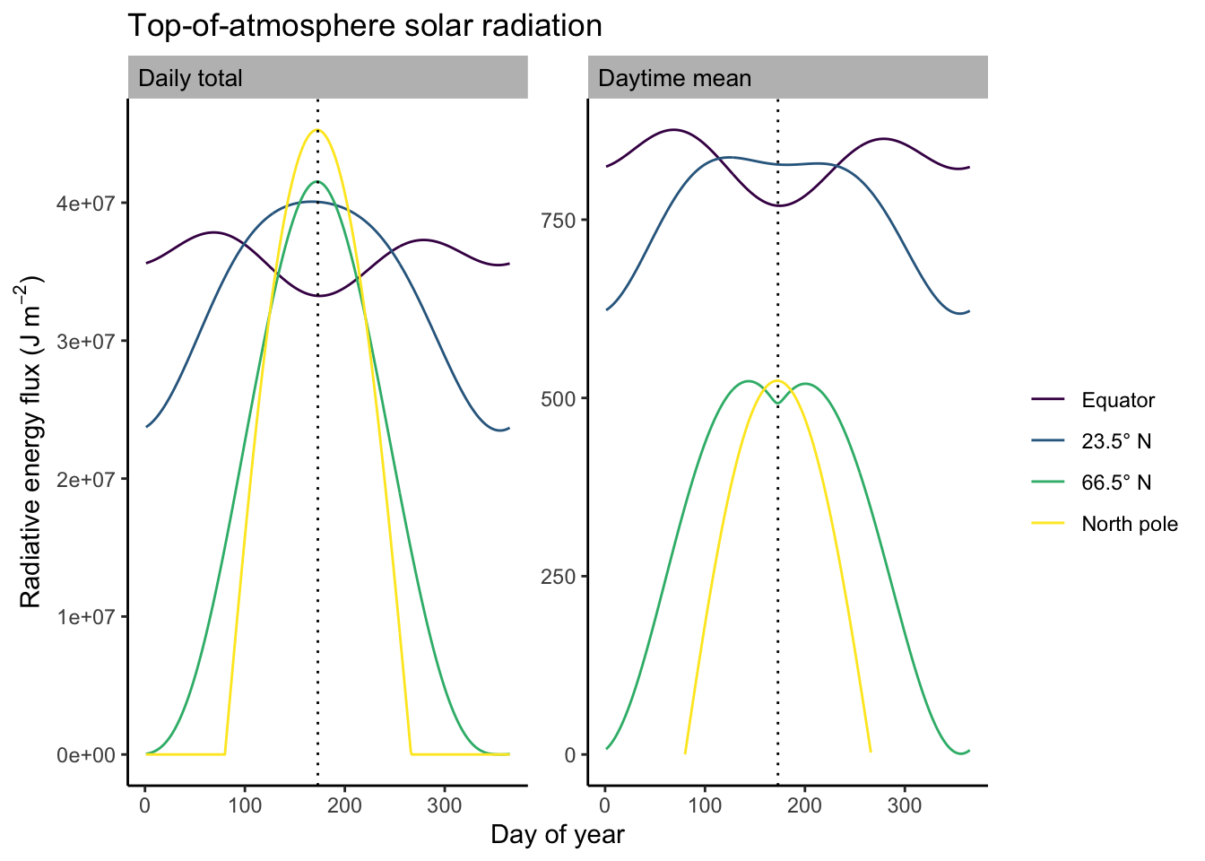
The areas under the curves in Figure 6.3 are proportional to the daily total solar radiation. Calculating daily totals involves a few integrals. The derivation is not shown here, but is explained in Davis et al. (2017). Daily totals and their variation over the seasons are shown below in Figure 6.4 and Figure 6.5.
Code
# use function calc_daily_solar() from Davis et al., 2017 GMD
source(here::here("R/solar.R"))

# Daily total and daytime-average S_TOA ---------------------
# for 4 different latitudes
df <- tibble(doy = seq(365)) |>
  rowwise() |>
  mutate(s_toa = calc_daily_solar(0, doy)$ra_j.m2,
         dayl = calc_daily_solar(0, doy)$hs_deg * 24.0 * 60 * 60 / 180,
         lat = 0
         ) |>
  bind_rows(
    tibble(doy = seq(365)) |>
      rowwise() |>
      mutate(s_toa = calc_daily_solar(23.5, doy)$ra_j.m2,
             dayl = calc_daily_solar(23.5, doy)$hs_deg * 24.0 * 60 * 60 / 180,
             lat = 23.5
             )
  ) |>
  bind_rows(
    tibble(doy = seq(365)) |>
      rowwise() |>
      mutate(s_toa = calc_daily_solar(66.5, doy)$ra_j.m2,
             dayl = calc_daily_solar(66.5, doy)$hs_deg * 24.0 * 60 * 60 / 180,
             lat = 66.5
             )
  ) |>
  bind_rows(
    tibble(doy = seq(365)) |>
      rowwise() |>
      mutate(s_toa = calc_daily_solar(90, doy)$ra_j.m2,
             dayl = calc_daily_solar(90, doy)$hs_deg * 24.0 * 60 * 60 / 180,
             lat = 90
             )
  ) |>
  mutate(s_toa_daily_avg = s_toa / dayl)

df |>
  rename(`Daily total` = s_toa, `Daytime mean` = s_toa_daily_avg) |>
  pivot_longer(c("Daily total", "Daytime mean"), values_to = "s_", names_to = "var") |>
  ggplot(aes(doy, s_, color = as.factor(lat))) +
  geom_line() +
  geom_vline(xintercept = 173, linetype = "dotted") +
  scale_color_viridis_d(
    labels = c("Equator", "23.5° N", "66.5° N", "North pole"),
    name = ""
  ) +
  labs(title = "Top-of-atmosphere solar radiation",
       x = "Day of year",
       y = expression(paste("Radiative energy flux (J m"^-2, ")"))) +
  theme_classic() +
  facet_wrap(vars(var),
             scales = "free") +
  theme(
    strip.background = element_rect(fill = "grey", color = NA),
    strip.text = element_text(color = "black", size = 10, hjust = 0)
  )
Code
# all combinations of day-of-year and latitude
df <- expand.grid(
  doy = seq(1, 365, by = 2),
  lat = seq(-90, 90, by = 2)
  ) |>
  rowwise() |>
  mutate(s_toa = calc_daily_solar(lat, doy)$ra_j.m2)

df |>
  ggplot(aes(x = doy,
             y = lat,
             fill = s_toa)) +

  geom_raster() +
  scale_fill_viridis_c(option = "magma") +
  coord_fixed(ratio = 1.2) +
  labs(title = "Top-of-atmosphere solar radiation",
       subtitle = "Daily total, year 2000",
       x = "Day of year",
       y = "Latitude (°N)",
       fill = expression(paste("J m"^-2))) +
  scale_x_continuous(expand = c(0,0)) +
  scale_y_continuous(expand = c(0,0))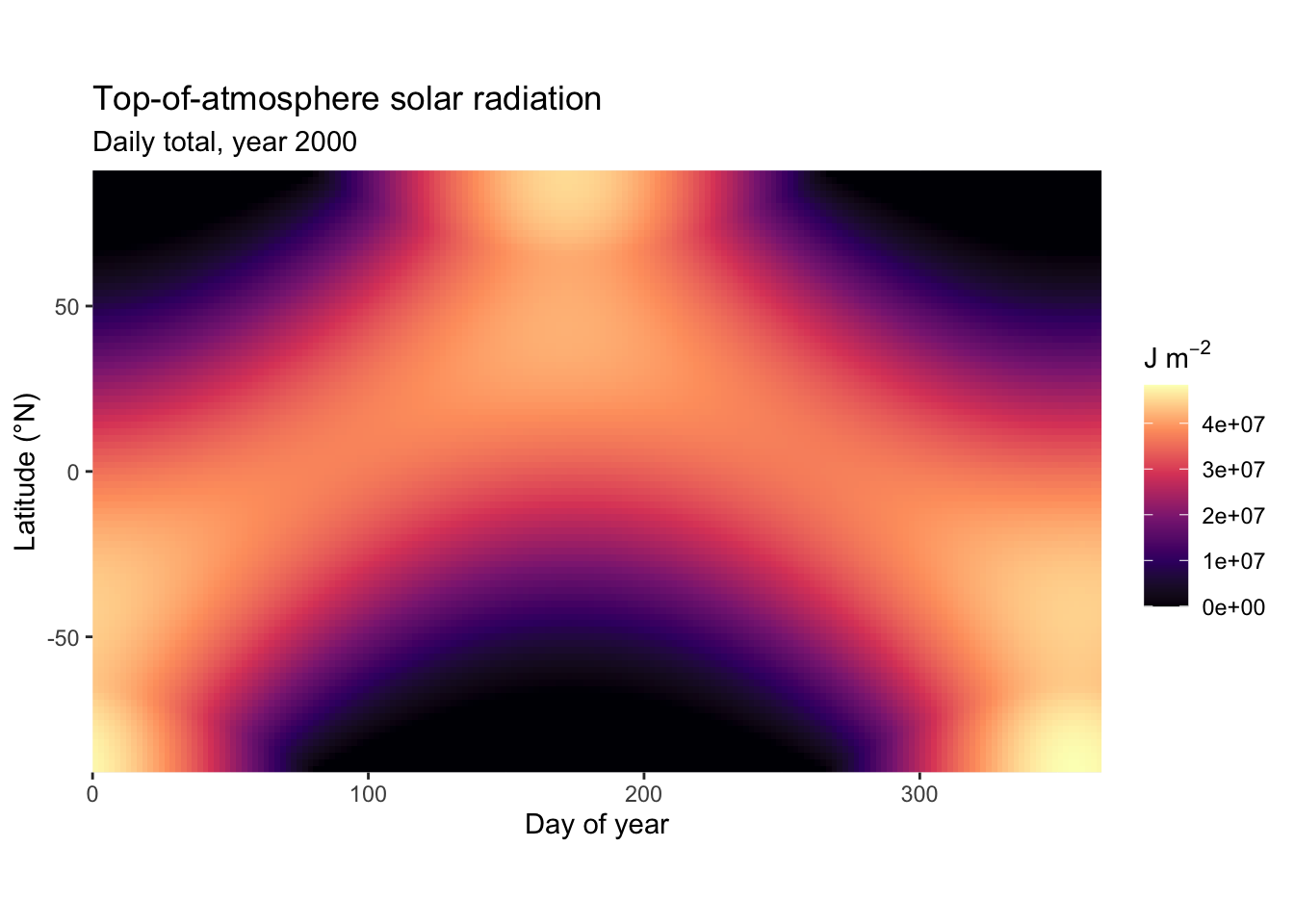
The diurnal (over the course of a day) and seasonal patterns in top-of-atmosphere solar radiation, following from solar geometry and expressed through Equation 6.4, have direct consequences for CO2 uptake patterns, as expressed through Equation 4.1, Equation 6.1, and Equation 6.3 and described further in Chapter 6.
Some features are particularly noteworthy about the patterns in \(I_\mathrm{TOA}\):
- The diurnal variation of the instantaneous flux is largest in the tropics.
- The seasonal variation of the daily total flux is largest at the North Pole.
- At the summer solstice, the daily total solar radiation is largest at the North Pole, …
- … but the daily maximum instantaneous and the daytime mean radiation flux are lower at the North Pole than at the equator at the summer solstice.
The biology of plants is attuned to the solar radiation patterns across different latitudes. The photosynthetic apparatus is constructed to make best use of the light, even during the hours of peak light intensity at mid-day. The phenological phases of plant growth reflect the light distribution over the seasons - evergreen plants dominate in the moist tropics to make use of the light year-round, while deciduous leaf strategies and annual life history strategies dominate in the northern latitudes where the seasonal fluctuation of light is large.
6.1.4 Long-term variations in solar radiation
Solar irradiance
The solar constant \(I_S\) isn’t actually constant but varies on the order of 0.1% of the course of a solar cycle. One cycle is approximately 11 years. The cyclic behavior is related to the periodic flip of the sun’s magnetic field and the number of sunspots. The radiation emitted from the sun and the number of sunspots are at their minimum after a magnetic flip. There is also a small long-term trend in the solar radiation, having increased by <0.1% since the Maunder Minimum (1645–1715). Solar irradiance is measured at high altitude to minimize the influence of the atmosphere (\(\tau\) in Eq. Equation 6.1) and get information about how \(I_S\) varies. Reconstructions of solar irradiance changes for the pre-instrumental period are based on the relationship between \(I_S\) and the (easily observable) sunspot number. Variations in \(I_S\) are small and do not have a dominant effect on climate and the carbon cycle that would override other forcings, especially for the industrial period (IPCC 2021).
Volcanic activity
Volcanic eruptions can influence the solar radiation at the Earth’s surface. Events that reduce solar radiation by more than 1 W m-2 occur approximately every 35-40 years (Gulev et al. 2021) and affect climate and the carbon cycle for up to a few years after very large eruptions. The increased aerosol load in the atmosphere reduces the total radiative energy flux (reducing \(\tau\) in Eq. Equation 6.1). However, through the strong positive effect of the aerosol load on the share of diffuse versus direct radiation, volcanic aerosols can affect the terrestrial carbon cycle, (somehow surprisingly) leading to a greater land C sink following years of large volcanic eruptions (Section 4.2).
Orbital parameters
The largest changes in \(I_\mathrm{TOA}\) arise over millennial time scales and are related to variations in Earth’s orbit around the sun. These Milankovic cycles are the trigger for the large climate swings between ice ages and warm periods over the course of ~100,000 years. Variations in the orbital parameters affect the latitudinal and seasonal distribution of \(I_\mathrm{TOA}\). Orbital parameters that vary periodically are:
- The eccentricity of the Earth’s elliptical orbit which affects the distance between the Earth and the sun, affecting \(I_\mathrm{TOA}\) via \(r_E\) in Equation 6.3. It varies with a period of approximately 100,000 years.
- The obliquity - the tilt of the axis of the Earth’s own rotation relative to the plane in which the Earth rotates around the sun. A greater obliquity amplifies seasonal variations in \(I_\mathrm{TOA}\). The obliquity is currently at 23.44°. At its minimum, it’s at 21.1°. Obliquity varies over 41,000 years.
- The precession is the rotation of the Earth’s own rotation axis itself. The effect of precession, in combination with the fact that the Earth’s orbit is elliptical, is that the variation of the sun-Earth distance shifts over the seasons. It varies with a period of about 25,700 years.
The point of minimal distance coinciding with the summer solstice leads to the largest mid-summer radiation maximum. As a result, the incident solar radiation over the northern-hemispheric summer at 65°N varied by about 83 W m-2 during the past million years. These changes are much larger than the ones driven by solar irradiance and volcanic activity.
About 6000 years ago, during the Mid-Holocene Warm Period, a summer maximum insolation for the northern hemisphere was reached (Figure 6.6). During this period, temperatures and solar irradiance during the growing season were elevated relative to the pre-industrial period and precipitation patterns shifted. This had profound effects on vegetation and the carbon cycle. Testimonies to this change are reconstructions that document a “Green Sahara” and a northward shift temperate and boreal forest biomes (MacDonald et al. 2000; Prentice, Jolly, and Participants 2000) during this period.
Code
# test:
# tmp <- purrr::map(seq(from = -300000, to = 2000, by = 500),
#                   ~calc_daily_solar(65, 173, year = .)) |>
#   purrr::map_dbl("ra_j.m2")

# all combinations of day-of-year and latitude
df_holo <- expand.grid(
  doy = seq(1, 365, by = 2),
  lat = seq(-90, 90, by = 2)
  ) |>
  rowwise() |>
  mutate(s_toa_holo = calc_daily_solar(lat, doy, year = -4000)$ra_j.m2) |>
  left_join(
    df,
    by = c("doy", "lat")
  ) |>
  mutate(diff = (s_toa_holo - s_toa))

df_holo |>
  ggplot(aes(x = doy,
             y = lat,
             fill = diff)) +
  geom_raster() +
  khroma::scale_fill_roma(reverse = TRUE) +
  geom_vline(xintercept = 173, linetype = "dotted") +
  coord_fixed(ratio = 1.2) +
  labs(title = "Mid-Holocene top-of-atmosphere solar radiation anomaly",
       subtitle = expression(paste("Daily total, ", italic(I)[TOA], "(6 kyr BP) - ", italic(I)[TOA], "(present)" )),
       x = "Day of year",
       y = "Latitude (°N)",
       fill = expression(paste("J m"^-2))) +
  scale_x_continuous(expand = c(0,0)) +
  scale_y_continuous(expand = c(0,0))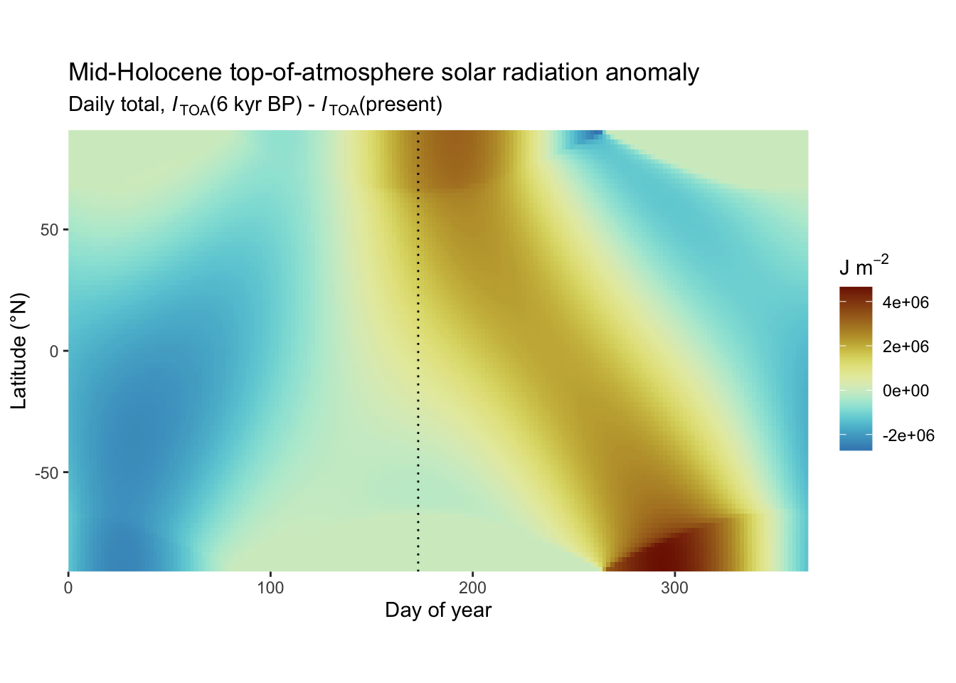
CautionExercise
- High solar radiation during summer drives monsoonal patterns in the tropics and sub-tropics. Considering Figure 6.6, how do you expect monsoonal precipitation intensity in the northern part of the African continent to have changed around 6 kyr BP, compared to today.
6.2 Phenology
In general, phenology refers to the study of periodic events of biological activity. In most cases, such periodic events are linked to the seasonal variations of the climate. In the context of terrestrial photosynthesis and land-climate interactions, the most important phenological event is the leaf unfolding and leaf senescence and shedding in response to seasonal variations in temperature, radiation, and water availability. The presence (or absence) of active green leaves has major implications for CO2, water vapor, and energy exchange between the land surface and the atmosphere.
The presence of green leaves is recorded by optical satellite remote sensing and documents the Earth’s greenness dynamics that follows the seasons - differently across the globe, as the video below illustrates.
CautionExercise
- Why does the “green belt” in Africa move north and south over the seasons?
Leaf phenology is either controlled by temperatures and light availability in temperate, boreal, and tundra ecosystems, or by water availability in warm, seasonally dry climates elsewhere. The water control on vegetation and leaf phenology will be discussed in Chapter 8.
In winter-cold climates (temperate, boreal, and tundra climate zones C, D, and E, see Figure 2.22), leaf phenology of deciduous plants is driven by the seasonal fluctuations of temperature and radiation. Leaves are shed before winter to avoid damage by cold temperatures and because the limited gains by C assimilation during dark and cold winter months does not outweigh the costs for maintenance of vital functions. In seasonally dry climates (mainly climate zones Am, Aw, see Figure 2.22), leaves are shed to avoid water loss and avoid dangerous desiccation of the plant. Leaf area also varies more gradually in response to seasonal variations in climate. LAI can have a seasonal cycle also in evergreen forests and shrublands. In grasslands, LAI typically has a strong seasonal cycle, with rapid foliage development and senescence during the typically relatively short vegetation period - but without the typical budbreak, leaf unfolding, and leaf shedding as in deciduous trees.
Photosynthesis and the exchange of CO2 between the land surface and the atmosphere are very directly affected by the amount of active green leaves - as measured by fAPAR (Equation 4.1). Coupled to this exchange is the exchange of water vapor and the surface energy balance. Therefore, leaf phenology is a primary control on land-climate interactions and the carbon cycle. Leaf phenology is not only a driver of land-climate interactions, but is also driven by climate. Different controls act on the leaf unfolding and leaf senescence dates.
6.2.1 Leaf unfolding
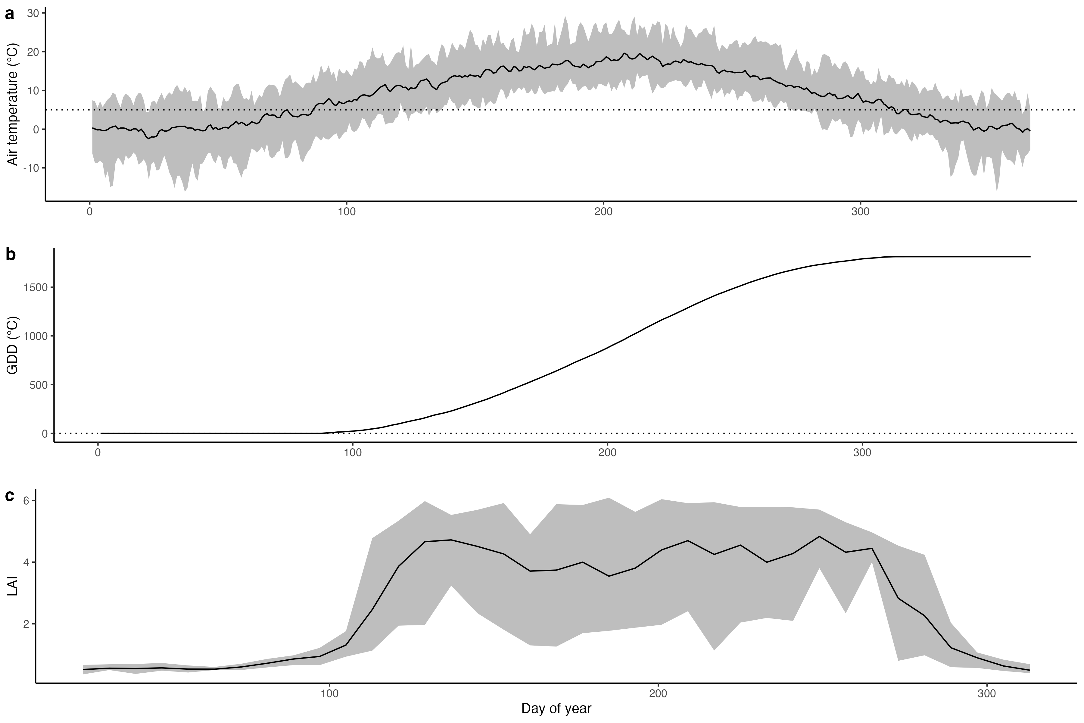
In winter-cold (temperate and boreal) deciduous forests, the timing of leaf unfolding (bud-burst) is sensitive to temperatures prior to the leaf unfolding date. Warm temperatures in early spring accelerate leaf unfolding and can lead to a shift of spring phenology dates by several days or even weeks. Phenology models commonly use the concept of growing degree days (GDD) (Basler 2016) and consider a critical GDD (GDD*) for predicting leaf unfolding. Growing degree days on day \(j\) is defined as the cumulative sum of temperatures above a specified threshold (\(T_0\), most commonly \(T_0 = 5^\circ\)C), counting from a given start date \(M\).
\[ \text{GDD}_{T_0,j}=\sum_{i=M}^j \max(T_i-T_0, 0) \] The leaf unfolding date is then modeled as the day at which GDD* is reached. In other words, the leaf unfolding is triggered by the accumulated “warmth”. The GDD concept is also commonly used for modelling crop development stages in crop models (distinguishing vegetative growth, seed filling, etc.). GDD* is assumed to be a constant in space and time but may be distinguished by tree species (some trees require a higher GDD - more “warmth” - to start leaf unfolding than others.)
More complex models consider also abiotic factors leading up to the phase (endodormancy, state of inactivity mediated by factor inside the bud, (Basler 2016)) where an increasing GDD drives bud development and leaf unfolding. For example, some models consider the requirement of a chilling phase - a period of cool, but non-freezing temperatures in the range of 2–7°C (Basler 2016) - and photoperiod (measuring the seasonal variation of daylength). However, complex models do not generally yield better predictive power than simple GDD-based models (Basler 2016). It should also be noted that models relying purely on temperature for modelling leaf unfolding may have limited applicability for simulating responses to long-term climatic trends. Plant-specific, biotic factors responding to photoperiod impose bounds on the sensitivity of phenology to temperature (Christian Körner and David Basler 2010).
Here in Switzerland, most trees start leaf unfolding in the second half of April. Why are leaves of winter-cold deciduous trees not unfolding earlier in the year (given that there is light available for photosynthesis)? Leaf shedding is a protection of plants against frost. At temperatures below freezing, costly cell protection measures against frozen water and excessive photosynthetic light harvesting are required to avoid damage. Delayed leaf unfolding is a strategy to avoid such damage.
Note
Check out our tutorial here to learn more about phenology modelling and fitting the GDD model to remotely sensed phenology data
6.2.2 Leaf senescence
Leaf senescence in temperate and boreal deciduous forests is - similarly as leaf unfolding - a strategy to avoid stress and damage by low temperatures in winter. Before leaf abscission (leaf shedding), the leaf nutrients are resorbed and photosynthetic activity starts declining. Leaves are rich in nutrients. A large fraction of nutrients contained in leaf biomass, in particular nitrogen (N), is linked to photosynthesis - mostly Rubisco. These nutrients are re-mobilised before leaf abscission and resorbed into plant-internal storage compartments. Thereby, the loss of “costly” nutrients can be avoided. A side effect of the nutrient resorption is the change of the leaf color to yellow, reddish, or brown.
Environmental controls on leaf senescence are not the same as for leaf unfolding and vary between tree species. Model predictability for leaf senescence dates is generally lower than for leaf unfolding dates, observed global trends are less clear (Piao et al. 2019), and drivers less well understood (Richardson et al. 2013) than for spring phenology. Photoperiod and temperature are considered important abiotic controls on leaf senescence dates. While photoperiod sets the induction of the end-of-season phenology, temperature modulates its progression with cold temperatures accelerating leaf senescence (Christian Körner and David Basler 2010). Also, the timing of leaf unfolding can appear to affect the timing of leaf senescence (Keenan and Richardson 2015; Marqués et al. 2023). An earlier leaf unfolding in spring appears to induce an earlier leaf senescence in autumn. Processes driving this pattern may be related to cell aging and a conserved leaf longevity, but may also be related to the ecosystem water balance and premature defoliation as a response to dry soil conditions (after vegetation has started consuming water earlier in spring).
6.2.3 Phenology trends and spatial patterns
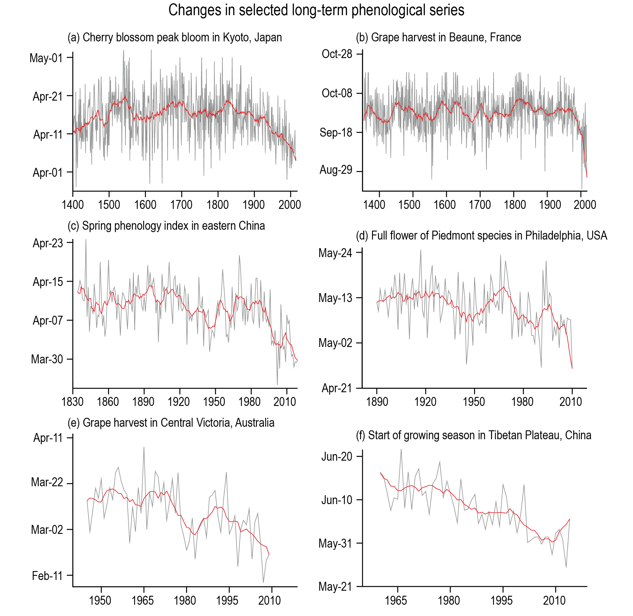
Since leaf unfolding and senescence phenology is sensitive to climate, patterns in spring phenology emerge across climatic gradients and over the course of long-term climate change. Phenology is very evident for an observer without technical instruments, and the timing of phenological dates can be relatively well determined. This has enabled the recording of phenological dates since centuries, and long-term phenological records now impressively document the unprecedented current warming in the context of the last few centuries Figure 6.8.
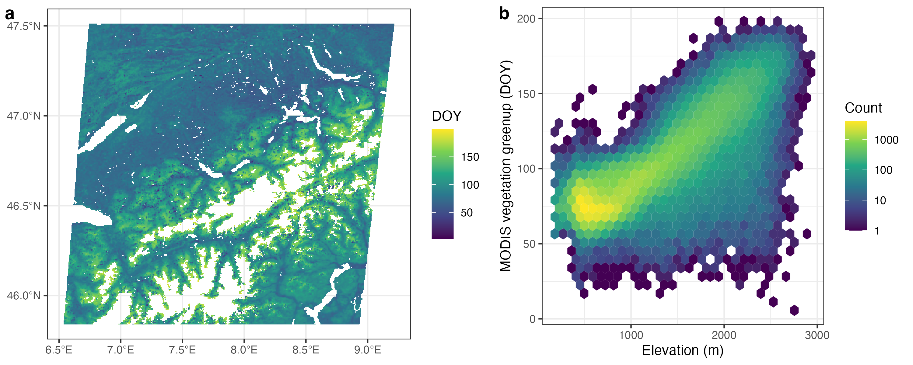
Variations in leaf unfolding dates are also evident across space, i.e., across climatic gradients in space. In mountainous regions, climatic gradients are steep and variations in the timing of leaf unfolding can be observed by eye - or from space across a larger region (Figure 6.9).
CautionExercise
- With rising temperature under anthropogenic climate change, how do you expect the risk of frost events causing damage on unfolded leaves to change?
6.3 Temporal variations of ecosystem C fluxes
Solar radiation is the “engine” of photosynthesis and thus of the terrestrial carbon cycle. This is expressed by the light use efficiency model of GPP (Equation 4.1). The temporal and spatial patterns of photosynthetic CO2 uptake are therefore driven by the temporal and spatial patterns in solar radiation. The Earth’s revolution around its own axis within a day, and its revolution around the sun within a year give rise to diurnal and seasonal variations in solar radiation, climate, C fluxes, and biological activity in all its forms. (It’s a fascinating thought that even physiological and psychological circadian rhythms like wake and sleep patterns are a consequence of solar geometry.) The variations of solar radiation over the course of a day and a year are expressed very differently along different latitudinal positions.
Note that both spatial and temporal variations in the photosynthetic CO2 uptake are driven not only by solar radiation, but are constrained also by water availability. The ecosystems for which fluxes are shown below (BR-Sa3, DE-Hai, FI-Hyy, and US-ICh, site locations are shown in Figure 2.2 and climate diagrams in Section 2.2) are all relatively moist and fluxes are rarely limited by water availability. An exception is the tropical forest site BR-Sa3 where months from August to October are relatively dry (Figure 2.3).
6.3.1 Diurnal cycle
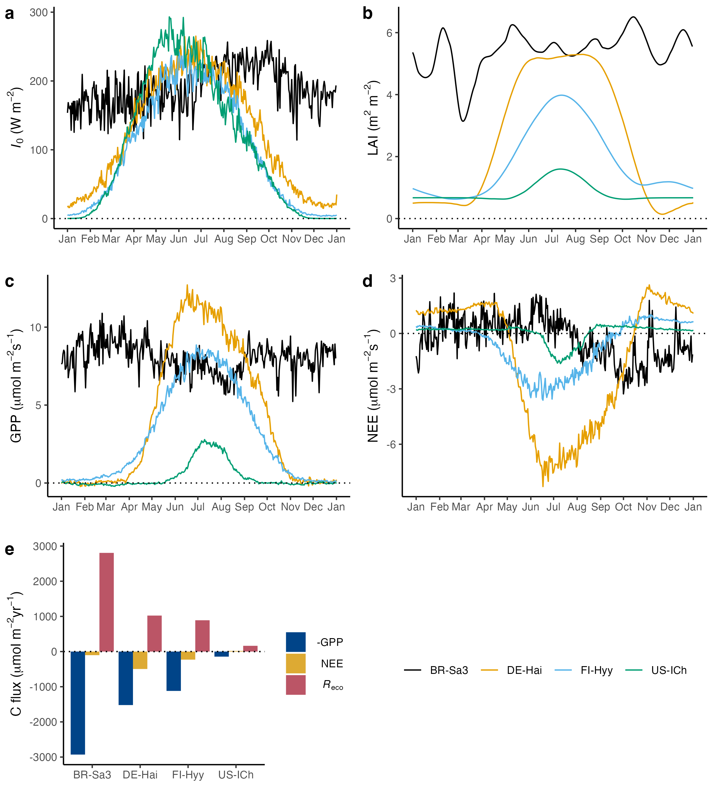
Figure 6.3 showed the diurnal cycle of the cosine of the solar zenith angle (\(\cos \theta_z\)) for different latitudes around summer solstice (21 June). \(\cos \theta_z\) is relevant because it linearly scales the top-of-atmosphere solar radiation, as described by Equation 6.3. The solar radiation incident at the Earth’s surface (\(I_0\)), that is at the top of the canopy, is shown for four different example sites in Figure 6.10. The same general pattern becomes evident:
- The sites at high northern latitudes (US-ICh, a tundra heathland in Alaska, and FI-Hyy, a boreal coniferous forest in Finland) have the smallest diurnal cycle amplitude in \(I_0\), but the longest daylight period (\(I_0 > 0\)).
- The low-latitude site in the tropics (BR-Sa3, a moist tropical forest) has the shortest duration of daylight (\(I_0 > 0\)), but reaches the highest mid-day solar radiation intensity. (Note that for \(I_\mathrm{TOA}\), a site at 23.5°N was shown in Figure 6.3 and has an even higher mid-day peak.)
- The temperate site (DE-Hai, a beech forest in Germany) is intermediate in terms of amplitude, peak value, and daylight duration.
The diurnal cycle in GPP (Figure 6.10 b) reflects the diurnal cycle in \(I_0\), but with some notable deviations:
- The mid-day peak for the tundra site US-ICh is much lower in relation to the mid-day peak of other sites for GPP than for \(I_0\). This is likely due to sparse vegetation cover (low LAI ad fAPAR) and temperature effects on photosynthesis.
- The shapes of the diurnal cycles in \(I_0\) and GPP are notably different for BR-Sa3. This may be an indication of water limitation on photosynthesis.
In the absence of disturbances influencing ecosystem C fluxes, the net ecosystem exchange (NEE) is largely equivalent to the negative of NEP as defined in Section 5.1.6. NEE is what the atmosphere “sees” - it is the net C flux between the atmosphere and the land surface (here a forest vegetation). A negative NEE value indicates a net CO2 uptake by vegetation. Some notable patterns in the diurnal cycle of NEE are:
- The diurnal cycle in NEE (Figure 6.10 d) is almost identical to the negative of the diurnal cycle in GPP. This reflects that variations in the net C balance of an ecosystem over the course of a day are strongly driven by photosynthetic CO2 uptake. Ecosystem respiration (Reco, the sum of autotrophic and heterotrophic respiration) varies less over the course of a day.
- Sites with a strong mid-day CO2 uptake have a higher night-time respiration.
- During nighttime hours, NEE is relatively stable. During that time, GPP is zero. Hence, Reco is relatively stable during the night.
- The daily total NEE (Figure 6.10 c) is smaller than daily totals in GPP and Reco. At the tropical site, NEE is very small in comparison to GPP and Reco. This indicates that over the course of one day, the tropical forest site is nearly C neutral. A substantial net C uptake is evident for DE-Hai. This is the C balance for a day in mid July. In general, during summer, temperate, boreal, and tundra ecosystems are a net C sink, and a net C source during winter (see Section 6.3.2).

6.3.2 Seasonal cycle
Figure 6.4 shows the seasonal cycle of top-of-atmosphere solar radiation (\(I_\mathrm{TOA}\)) for different latitudes. The daily totals exhibit the same general seasonal pattern as measured incident top-of-canopy solar radiation means, measured at four different sites along different latitudes (Figure 6.11):
- The seasonal cycle amplitude is smallest at low latitudes (at the Equator for \(I_\mathrm{TOA}\) and site BR-Sa3 for \(I_0\)) and highest at high latitudes. Daily solar radiation drops to zero in the Arctic during winter north of the Arctic circle at 66.5°N. (FI-Hyy is located at 61.8°N, US-ICh is located at 68.6°N).
- Mid-summer peak daily solar radiation is highest at high northern latitudes (at the North Pole for \(I_\mathrm{TOA}\) and at site US-ICh for \(I_0\)).
- The small seasonal variation in \(I_\mathrm{TOA}\) at the Equator does not translate into congruent seasonal variation in \(I_0\).
A similar overall pattern is visible for the seasonal variation in GPP, but with some notable exceptions:
- The highest seasonal peak daily GPP values are recorded at the temperate site DE-Hai. This is despite LAI being mostly higher at the tropical (BR-Sa3) than at the temperate site and indicates a very high mid-summer LUE of ecosystem photosynthetic CO2 uptake at the temperate site.
- The mid-summer peak daily GPP is (by far) lowest at the tundra site US-ICh. This reflects the very low LAI at this site.
- The (deciduous) temperate forest site DE-Hai - a beech forest in Germany - exhibits the largest seasonal variation in LAI. Beech is a deciduous tree and forms forests that are strongly dominated by beech alone with little understorey vegetation. The simultaneous leaf phenology of the dominating tree species drives the rapid and large spring increase and autumn decrease in LAI.
- FI-Hyy is a needle-leaved forest, dominated by pine trees (Pinus sylvestris and Picea abies). Although these tree species are evergreen, a seasonal variation in LAI is recorded by the satellite remote sensing-derived observations shown in Figure 6.11 (b). This likely reflects three aspects: (i) the small but not absent actual seasonal variation in leaf area also in evergreens, (ii) the influence of the deciduous understorey vegetation on ecosystem-level greenness, (iii) the snow cover during winter months affecting the remotely sensed signal in surface reflectance which is interpreted by the algorithm for estimating LAI.
As for the diurnal cycle, also for the seasonal cycle, the pattern in NEE strongly resembles the negative of the pattern in GPP. Some notable aspects are:
- The tundra (US-ICh) and boreal (FI-Hyy) sites are small sources of CO2 during winter and moderate sinks in summer.
- The temperate site DE-Hai is a substantial sink in summer and a moderate source in winter. The peak of the source is attained in the shoulder seasons (April and November) - when temperatures are still above freezing and drive respiration, while leaves are already shed or not yet unfolded.
- The annual total NEE is small for all sites and nearly zero for the tropical and the tundra sites (BR-Sa3 and US-ICh, respectively). The small NEE is the net of the two much larger opposing fluxes GPP and Reco.
CautionExercise
- At what latitude do you expect the largest diurnal cycle amplitude in top-of-atmosphere solar radiation?
- At what latitude do you expect the largest seasonal amplitude in top-of-atmosphere solar radiation?
- Where do you expect the smallest seasonal variation in the daily net ecosystem productivity?
- Consider mature forest ecosystems (sensu Odum (1969), Figure 5.7) in a moist tropical, temperate and boreal region. Where do you expect the largest annual NEP? Where do you expect the largest daily NEP during the peak growing season?
6.3.2.1 The breathing of the Earth
The NEE (equivalent to the negative of NBP, introduced in Section 5.1.6) recorded at the four example sites shown above is representative for similar patterns across all vegetated land of the Earth. Seasonal variations in solar radiation are the underlying driver of the carbon flux variations and similarly affect all photosynthesizing organisms across the planet.
CO2 is relatively well-mixed in the atmosphere due to its long lifetime. However, the mixing time scale is on the order of a couple of years. Hence, more rapid variations in net CO2 fluxes between the atmosphere and the Earth surface (over the ocean and over the land) are expressed in corresponding variations of the atmospheric CO2 concentration. As introduced in Section 1.1.1, the atmospheric CO2 concentration, measured at Mauna Loa (Hawaii) exhibits not only a steady increase since the 1950s, but also a seasonal cycle with the lowest value at the end of the northern hemisphere summer. Atmospheric CO2 is continuously measured at a range of sites along different latitudes. At Point Barrow, the northernmost point of the US in Alaska, the CO2 seasonal amplitude is even larger than at Mauna Loa (Figure 6.12). This is the result of the collective net CO2 uptake in northern ecosystems during summer.
Figure 6.12 shows the seasonal variation in atmospheric CO2 after the mean and long-term trend are removed from the time series (corresponding to the red curve minus the black curve in Figure 1.1). The shape of this seasonal variation is very similar to the shape of the seasonal NEE variation at northern sites (e.g., DE-Hai) - above average during winter months when ecosystem respiration prevails and a rapid draw-down starting in spring to attain a minimum during summer. This shows how the patterns in net ecosystem CO2 exchange directly affect variations in atmospheric CO2 over the course of a year.
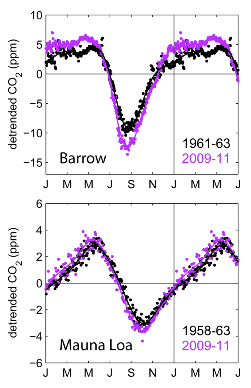
Figure 6.12 also shows that the CO2 seasonal amplitude has been increasing since measurements started in the early sixties of the 20th century. This increase reflects changes in the terrestrial C cycle (Graven et al. 2013) and is likely driven by the warming climate and the extension of the growing season in northern ecosystems, increasing the photosynthetic CO2 uptake as a result of the fertilizing effect of rising CO2, and seasonal shifts in GPP and Reco and their relative timing.
The video below shows an animation of the modeled spatial and temporal variations of atmospheric CO2 over the course of one year. CO2 sources from fossil fuel combustion by industry, households, and traffic are combined with the modeled terrestrial and oceanic net CO2 exchange between the Earth’s surface and the atmosphere. An atmospheric transport model is then used for simulating variations in CO2 concentrations.
6.4 Spatial variations of ecosystem C fluxes and stocks
C fluxes between the a land ecosystem and the atmosphere vary over the course of a day and over the course of a year, as described above in Section 6.3. Annual totals vary relatively little between years (not shown). However, annual total C uptake and release fluxes vary very strongly across different geographical locations, climates and types of ecosystems. As much as solar radiation is the driver of temporal variations in photosynthetic CO2 uptake, it is also a strong driver of its spatial variations across the globe.
6.4.1 Terrestrial primary productivity patterns
Once more, the light use efficiency model (Equation 4.1) serves as a guide for understanding the drivers of spatial patterns in terrestrial GPP. In this subsection, we follow the study by Wang, Prentice, and Davis (2014) and estimate the magnitude and global distribution of GPP by successively considering physical and physiological constraints on CO2 assimilation.
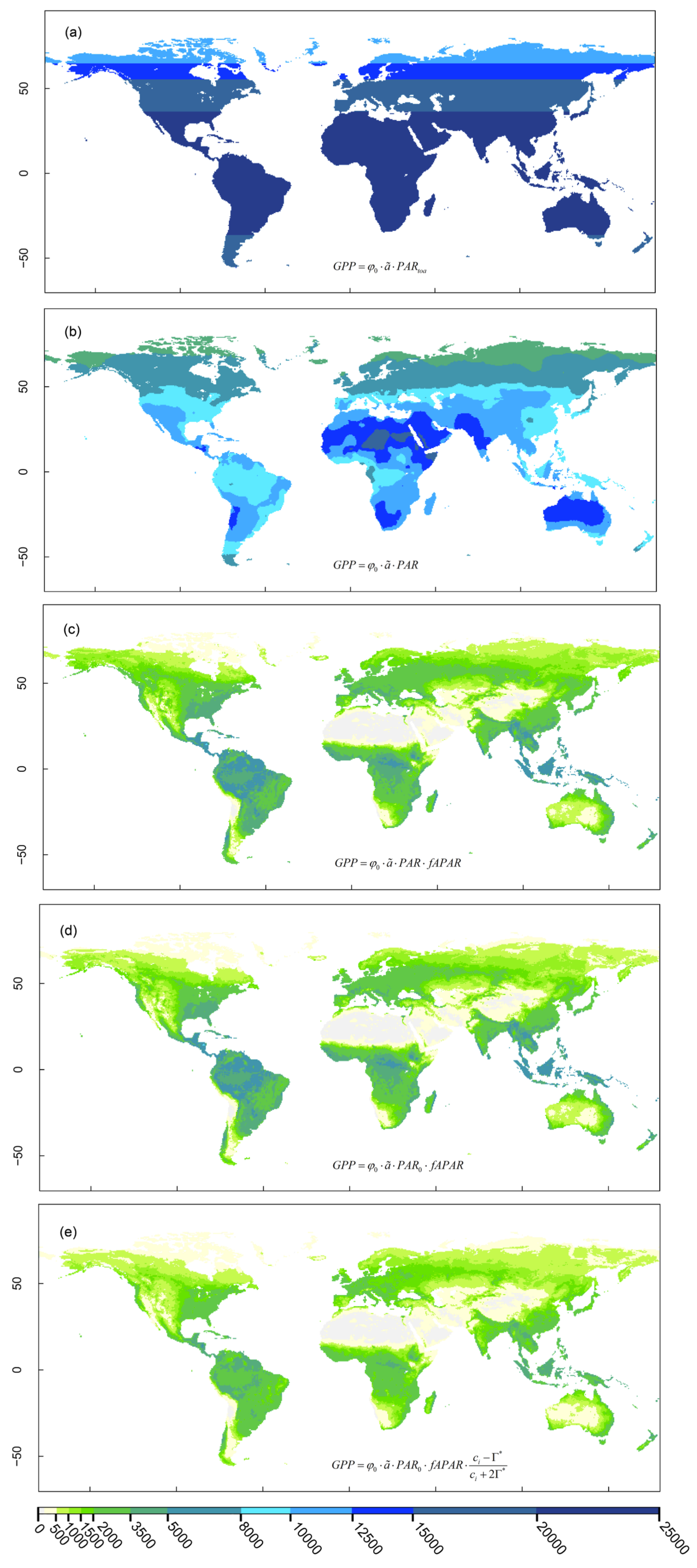
We start by adopting the hypothetical perspective from the top of the atmosphere (TOA). We estimate the geographic pattern of terrestrial photosynthesis if the full energy of solar radiation received at the TOA was used for photosynthetic CO2 assimilation (Figure 6.13 a). In this case, GPP is equal to the product of the quantum yield (\(\varphi_0\)), a factor \(\tilde{a}\) that accounts for the incomplete utilization of absorbed light by the light reactions, and the photosynthetically active radiation received at the top of the atmosphere (PARTOA in Figure 6.13, corresponds to ITOA in Equation 6.1). In this (hypothetical) case, the global distribution of GPP varies along latitudes, but not along longitudes and is estimated by Wang, Prentice, and Davis (2014) at 2960 PgC yr-1.
Next, we consider the attenuation of solar radiation by the atmosphere, considering cloud cover and the elevation of the land surface. This considers Equation 6.2 and reflects the geographic pattern of distribution of solar radiation, incident at the land surface (Figure 6.1). Note that \(\varphi_0\) and \(\tilde{a}\) are considered here to be global constants. Atmospheric attenuation of photysnthetically active solar radiation reduces terrestrial GPP by over 50% (from 2960 to 1442 PgC yr-1, Wang, Prentice, and Davis (2014)).
Not all solar radiation that reaches the land surface is absorbed by active green vegetation. The highest radiation intensities coincide with sparsely vegetated land, including major desert regions. The effect of reduced vegetation cover on GPP is quantified by the factor fAPAR which accounts for the fraction of absorbed photosynthetically active radiation (Section 4.2). Limited vegetation cover and light absorption reduces terrestrial GPP further by over 75% (from 1442 to 322 PgC yr-1, Wang, Prentice, and Davis (2014)).
At the global scale, temperature has a relatively weak effect on GPP. Considering that photosynthesis is inhibited by freezing temperatures (below 0°C) does not substantially reduce total terrestrial GPP (from 322 to 300 PgC yr-1, corresponding to a 7% reduction, Wang, Prentice, and Davis (2014)). This is because low temperatures coincide with low PAR (or \(I_0\)). Situations of high light and low temperatures are relatively rare.
Finally, physiological effects of CO2, temperature, vapor pressure deficit, and the atmospheric pressure are considered. Note that the effect of temperatures below freezing is treated separately by the step described above. The potential maximum rate of the conversion of absorbed photosynthetically active radiation is reduced by the limited diffusion rate of CO2 through stomatal openings (thus reducing \(c_i\) relative to \(c_a\), Figure 6.13 e) and is further reduced by the effects of photorespiration as accounted for by the factor \((c_i - \Gamma^\ast)/(c_i + 2\Gamma^\ast)\). This represents the effect of leaf-internal CO2 concentration on the electron transport-limited assimilation rate \(A_J\) in the FvCB model (Equation 4.9). These physiological effects reduce terrestrial GPP from 300 to 211 PgC yr-1, corresponding to a 30% reduction (Wang, Prentice, and Davis 2014). Note that the range of published total annual terrestrial GPP estimates is lower - between 110 and 140 PgC yr-1 (Benjamin D. Stocker et al. 2019).
CautionExercise
- Which of the factors described above implies the strongest reduction in GPP? What resource limitation may be responsible for this large unrealised C assimilation?
6.4.2 Global distribution of biomass carbon
As explained in Chapter 5, photosynthesis is the ultimate source of all C cycling in ecosystems and accumulating in different pools along the C cascade - from live vegetation to litter and soil organic matter. Variations in GPP thus affect all “downstream” fluxes and pools along the C cascade. A reflection of this is the similarity in the global patterns of GPP and aboveground biomass C (Figure 6.14). In Chapter 5, we considered the C cascade and simulated the dynamics of all pools and fluxes in response to a change in GPP. We showed that, assuming that allocation, SOM partitioning factors, and pool-specific turnover times are constant, GPP linearly scales all downstream fluxes and pools. We also noted that in reality, allocation, SOM partitioning, and turnover times cannot be assumed constant over time. When considering variations across space - across different climates, soils, and ecosystem types - constancy in these factors is probably an even less justified assumption.
While Figure 6.14 shows an overall similarity between the patterns of GPP and aboveground carbon, it’s also instructive to consider the deviations. Aboveground biomass is by far largest in tropical forest regions. While temperate forest regions attain annual GPP of a similar magnitude as tropical forests (Figure 6.13 e), their aboveground biomass is substantially lower. Even more discrepant are differences between forest versus savannah and grassland regions. While the extent of the tropical forest biome in Africa is clearly reflected by the distribution of aboveground biomass and shows a sharp transition to much lower values at its margins, such a sharp transition is not visible for GPP (Figure 6.13 e). This indicates that grasslands and savannahs can be highly productive, but if assimilated C is not used for wood production, then their high productivity is not translated into high biomass stocks. This aspect is also explained in Section 5.1.3 where the difference in C allocation between forest and grasslands is described and quantified (Table 5.1).
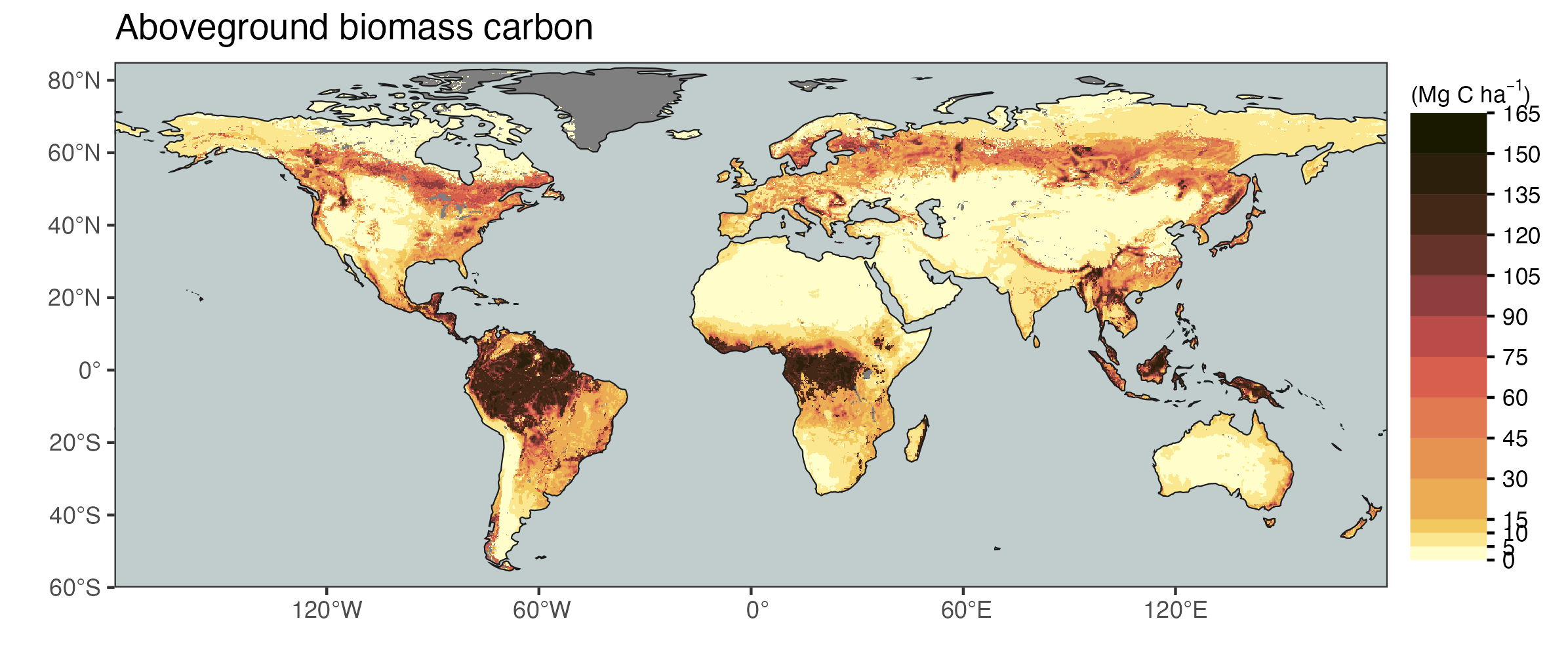
While the global biomass map in Figure 6.14 shows the overall pattern of highest aboveground biomass C being located in tropical forests, it hides “pockets” of exceptionally high biomass in temperate forests. Some of the world’s highest biomass densities (average biomass per unit ground area in a forest plot) are found in cool and moist temperate forests, including Eucalyptus regnans-dominated forests in southeast Australia, Sequoia-dominated forests in coastal California, Oregon and Chile, and Agathis australis-dominated forests in New Zealand (Keith, Mackey, and Lindenmayer 2009).
6.4.3 Global distribution of soil carbon
In Section 5.1.5, we conceived soil C dynamics as a first-order decay process. This assumes that the soil C stock scales linearly with the C inputs. C inputs are determined by litter production which, at long enough time scales, is equal to biomass production which, in turn, is correlated with GPP (Figure 5.3). In summary, a first-order decay model for SOM would predict that soil C stocks scale with GPP and the global distribution of soil C would be similar to the global distribution of GPP (Figure 6.13 e).
However, Figure 6.15 shows that the pattern of the global soil C distribution is markedly different from the global pattern of GPP. This suggests that C inputs alone are not a good predictor of soil C stocks. Other factors play important roles, as described below. Note however that in unproductive desert regions, also soil C is low.

Controls on soil C stocks
Allocation Root inputs are approximately five times more likely than an equivalent mass of aboveground litter to be stabilized as soil organic matter (SOM) (Jackson et al. 2017). Thus, allocation and plant growth in different tissues is an important factor determining the link between vegetation productivity, litter production, and soil C. In grasslands and shurblands, a much larger fraction of C is allocated to roots than in forests. Thus, soil C stocks are often higher in natural grasslands and shrublands than in forests. This is also visible in Figure 6.15 which indicates high soil C stocks in the Earth’s grassland and shrubland-dominated regions.
Climate The activity of soil organic matter-decomposing microbes (fungi and bacteria) is strongly controlled by abiotic factors in the soil. Under low temperatures, their activity is reduced, and soil and litter decomposition rates are slowed (see also Section 5.1.5). This is reflected in Figure 6.15 by the generally high soil organic C stocks in the cold climates of the high northern latitudes - despite the generally low productivity of vegetation in these regions.
Soil mineral composition Stabilisation and saturation of soil organic C depends on the mineralogy of the soil. This suggests that not (only) the C inputs determine stocks, but also the capacity of soil mineral surfaces to adsorb organic matter.
Plant-soil interactions Plant-soil interactions via fungi and bacteria strongly influence C and nutrient cycling in soils. Inputs of fresh litter and labile C through root exudates can stimulate the decomposition (priming) of stable C in the soil. These relationships are complex and implications for the global distribution of soil C is not clear, but can undermine a positive and linear relationship between vegetation productivity, litter inputs, and soil C stocks.
Global soil C stocks
The total C stock in soils up to 2 m is estimated 2273 PgC by Jackson et al. (2017) - higher than the number provided in the IPCC AR6 (Canadell et al. 2021) and Figure 3.1. Global soil C estimates are based on soil organic C content measurements which are available mostly from the top soil and are thus sensitive to assumptions regarding the soil C distribution across the soil profile. In general, the organic matter and thus soil C content declines with depth but the rate of decline depends on vegetation and the distribution of roots. The global soil C stock of 0-3 m is even higher and estimated by Jackson et al. (2017) at 2800 PgC. The soil depth-to-bedrock puts a constraint on soil C storage at depth in many places, which is very uncertain, and may lead to a substantial reduction of the total 0-2 and 0-3 m soil C estimates.
The high soil C density in high northern latitudes (Figure 6.15) reflects also the particular functioning and soil C dynamics and stabilization under conditions where temperatures are below freezing for a large part of the year (in permafrost regions) and under permanently water-logged soil conditions (in peatlands). Contributions of soil C stocks in peatland and permafrost regions are substantial (see Section 6.4.4 and Section 6.4.5).
6.4.3.1 Link to biomass C distribution
Taken together, the global distribution of soil C deviates strongly from the distribution of GPP and biomass C. The parallel trends of average biomass and soil C along latitudes is shown in Figure 6.16 and illustrates the divergence of their latitudinal patterns. It should be noted that grasslands are typically very soil C rich due to the high allocation to fine root production as discussed above. Yet, aboveground biomass is low in grasslands compared to forests. This largely explains the pattern in Figure 6.16.

6.4.4 Peatlands
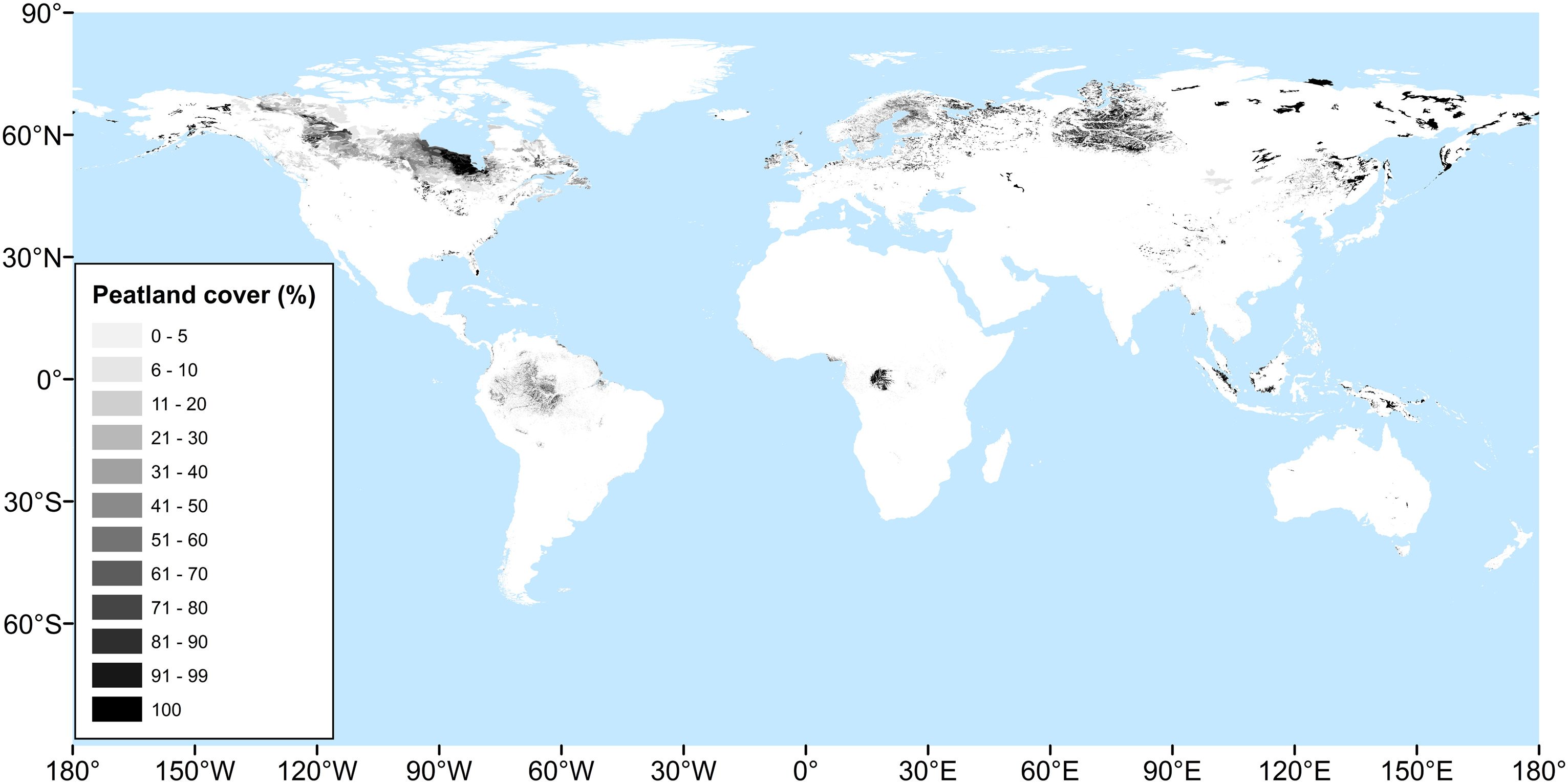
Under well-drained soil conditions, the organic carbon content of soil tends to stabilise during soil development. At this stage, on average over long time scales, decomposition of organic matter equals litter inputs. A steady-state is reached. However, decomposition by heterotrophic organisms requires oxygen. Under frequent flooding and water-logged soil conditions, oxygen availability becomes limiting for heterotrophic activity and decomposition is strongly reduced. If a long-term imbalance of vegetation productivity and litter inputs vs. decomposition persists, undecomposed litter C can accumulate. Peat and organic soils (histosols) form. Such conditions are given in very particular locations across the globe (Figure 6.17).
Peatlands are extremely C-rich, containing 500-700 PgC on only 3% of the Earth’s land surface (Page and Baird 2016; Yu et al. 2010). Collectively, peatlands across the globe are also a persistent C sink. Due to their special role in the C cycle, we afford a small excursion into the special world of peatlands.
NoteDefinitions
- Peat is the material that constitutes soils in peatlands.
- Peatland is a type of wetland where peat is present.
- Bog is a nutrient-poor type of peatlands.
- Raised bog (ombrotrophic bog, German: Hochmoor) is a bog in which organic matter has accumulated vertically to a degree such that plants with their roots are disconnected from the water table and receive nutrient inputs solely from atmospheric wet and dry deposition. Raised bogs are extremely nutrient-poor, acidic, and are dominated by mosses (sphagnum).
- Fen is a more nutrient-enriched type of peatland, is more alkaline, and dominated by sedges and grasses, but can also host shrubs and sparse trees. Plants growing in fens have access to water that has been in touch with mineral soils and bedrock and contains dissolved minerals. Hence, fens are referred to as minerotrophic.
Peatland distribution
In view of the frequent flooding and wet soil conditions, peatlands are considered a type of wetland. They occur in a wide range of biomes. In the tropics, decomposition rates - even under water logging - are much higher than in the Arctic. Yet, vegetation productivity is much higher, too, and can lead to an imbalance of organic matter inputs and decomposition and a long-term accumulation.
Today, major peatlands are located in the Hudson Bay Lowland (Canada) and in the West Siberian Lowland (Russia). In the tropics, major peatlands are located in Southeast Asia (Indonesia, Malaysia, Papua New Guinea, and Brunei) (Page and Baird 2016) and in the Congo Basin (Dargie et al. 2017). Peatland vegetation is very different in boreal and temperate versus tropical peatlands. The latter occurs in forested, often palm-dominated swamps and in coastal mangroves (Page and Baird 2016). Boreal and temperate peatlands are dominated by sedges or mosses (see box above).
Peatland establishment
The particular pattern of the global distribution of peatlands (Figure 6.17) reflects the environmental constraints on their development. This can be understood as a sequence of criteria that need to be fulfilled for the establishment of a peatland (B. D. Stocker, Spahni, and Joos 2014):
- Hydroclimate: The balance of mean annual precipitation (MAP) should be higher than the mean annual potential evapotranspiration (PET, see Chapter 8). PET measures how much radiation is available for evaporating water. A positive ratio of MAP/PET indicates a wet hydroclimate and is a primary prerequisite for the establishment of a peatland.
- C balance: Under water-logged conditions, vegetation productivity and litter inputs must outpace soil organic matter decomposition and a long-term C accumulation is necessary to form peat.
- Topography and soil drainage: Water-logged soil conditions and a shallow groundwater table depth are present in the landscape where subsurface water flow converges and where drainage is hindered either due to the topographic situation or due to impermeable soil layers or bedrock. Frequent conditions with the groundwater table near the surface or above (inundation) thus occur in low-lying depressions or in poorly drained plains, but less in convex terrain (e.g, ridges).
Peat growth
Peat is undecomposed plant material. Most of this material accumulates at the surface. In sphagnum-dominated bogs, all of this material accumulates at the surface since sphagnum forms no roots. Hence, peat grows vertically. Eventually, peat domes form and the peatland transitions to becoming a raised bog (see box above).
Peat layers form in each year by added litter, are subsequently covered by the next layer, and slowly decay over time, losing mass and volume. The oldest peat is found at its base, the youngest at the top. Due to the age-depth relation, peat soils also serve as a paleo archive.
Peatland history
Due to the very slow decay, the oldest peat present at a peat dome’s base may date back millennia. Indeed, dated carbon in peatlands across the globe indicates a peak in the initiation of northern peatlands in the early Holocene around 11-9 kyr BP and of tropical peatlands even before - around 20 kyr BP (Yu et al. 2010; MacDonald et al. 2006). The timing of the rapid initiation of northern peatlands coincides with the retreat of the major ice sheets after the Last Glacial Maximum and with a peak in summer insolation (Figure 6.6 and Figure 6.18) and climate seasonality with warm summers in the northern hemisphere, supporting vegetation growth. As new peatlands formed in the early Holocene, old ones that established in the glacial climate disappeared due to climatic change (Müller and Joos 2020) and were lost to rising sea levels during the melting of the ice sheets (Dommain et al. 2014).

Peatlands and the global carbon cycle
As mentioned above, peatlands store 500-700 PgC (more than all biomass C globally) on only 3% of the Earth’s land surface (Page and Baird 2016; Yu et al. 2010). Since the majority of the peat present today has accumulated over the course of the Holocene, an average C sink of >5 PgC (100 yr)-1 has persisted over the same duration (Yu et al. 2010). This is much smaller than the global fluxes of the anthropogenic C cycle perturbation, as quantified by the global carbon budget in Chapter 3. Yet, its persistent nature and the magnitude of long-term C accumulation has had implications for millennial-scale terrestrial carbon storage changes and atmospheric CO2 (B. Stocker et al. 2017). Due to their susceptibility to hydro-climatic conditions, peatland extent, global distribution, and C storage will likely undergo changes in a future climate. However, current research and model projections indicate unclear trends (Qiu et al. 2022).
Peatlands, as all wetlands, are also a major source of methane (CH4). Under anoxic soil conditions, CH4 is produced, rather than C being oxidized and CO2 released (Chapter 12).
CautionExercise
- Water table variations affect the C balance of a peatland. If it falls, how do you expect NPP, Reco, and NEP of a peatland, and the turnover time of C in soil organic matter to change?
- What other greenhouse gas may be influenced by a declining water table in a peatland? In what direction would its emission change?
- Why are soils dark in the Seeland of the Canton of Bern?
- Why are wooden artefacts of the Bronze age preserved in some places but not in others? Do you know any such wooden artefacts?
6.4.5 Permafrost
About 24% of the northern hemisphere’s exposed land surface contains ground that remains frozen for at least two consecutive years - the definition of permafrost (Schuur and Mack 2018). The global distribution of permafrost in the northern hemisphere is shown in Figure 6.19. Organic matter in frozen soils is protected from decomposition - as long as the ground remains frozen. The total amount of C stored in permafrost soils (0-3 m depth) is estimated at 1,035 ± 150 PgC (Tarnocai et al. 2009; Hugelius et al. 2014) and substantial additional C (400-500 PgC) is stored at greater depth in particular locations (river sediments) (Schuur and Mack 2018). This amount of C adds another 50-100% to the total amount of C stored in soils (Figure 3.1) and suggests that the distribution of permafrost is an important determinant for the global distribution of soil C (Figure 6.15).

Permafrost occurs (roughly) where the mean annual temperature is below freezing. During summer, the upper soil layers, the active layer, thaw. However, the seasonal fluctuation of soil temperature is attenuated deeper in the soil due to constraints on the rate of thermal diffusion across the soil. At a certain depth, the seasonal cycle of soil temperature disappears, and the soil temperature is largely constant and equal to the mean annual air temperature on the ground (\(Z^\ast\) in Figure 6.20). Towards greater depth, the temperature increases again due to the geothermal heat flux. Permafrost is the zone where temperatures never rise beyond 0°C.

The presence of permafrost constrains the volume available for plant rooting, vegetation access to water and nutrients, and the heterotrophic activity if microbes. It also prohibits the infiltration of water into deeper layers which can lead to a perched water table, water-logging, and anoxic conditions in the soil.
With rapid warming in northern high latitudes, permafrost temperatures are rising throughout the Arctic (Biskaborn et al. 2019). Implications of permafrost melting for greenhouse gases (CO2 and CH4) and the climate-land Earth system feedback are discussed in later chapters.
CautionExercise
- Why does the melting of permafrost affect methane emissions?