
5 Ecosystem carbon dynamics
In Chapter 3, we conceived the global carbon cycle as a system of three pools (atmosphere, land, ocean). The C dynamics in the land biosphere were modeled using a 1-box model which receives C inputs through photosynthesis and loses C through a constant turnover. In Chapter 4, we focused on the processes driving terrestrial CO2 uptake. In this chapter, we are unboxing the 1-box model and introduce the processes that determine C flows in ecosystems and their C balance. We will describe the C dynamics of an ecosystem, not as a single box with a single and constant turnover, but as a cascade of C, made of multiple pools with different turnover rates, and where the partitioning (allocation) of the cascading C into the different pools is influenced by the environment and by the ecosystem state.
5.1 Ecosystem carbon flows and pools
At the ecosystem-level, C dynamics can be described as the flows (fluxes) between carbon pools that represent C in non-structural forms, leaves (foliage), (stem) wood, fine roots, litter, and soil (Figure 5.1). C is respired by plants (autotrophic respiration) and by soil microbes (heterotrophic respiration). C in live vegetation biomass is turned over to produce litter (litterfall) as trees shed their leaves and lose branches (over years) and as they die (over decades to centuries). Plant mortality is related to the size and age of a tree and may be driven by disturbances (fire, pests, extreme drought and heat). Within years, litter is respired or transformed into soil organic C where it may be stabilized for centuries and more. Heterotrophic respiration originates from litter and soil C decomposition by microbes (fungi and bacteria).
5.1.1 Non-structural carbon and autotrophic respiration
C assimilated by photosynthesis is initially present as non-structural C (NSC) in the form of hydrocarbons (sugars). Some of the assimilated C is stored internally in the form of starch to fuel the reserves pool. Some of the assimilated carbon is consumed by autotrophic respiration (\(R_a\)) which subsumes different processes, including maintaining vital functions of the plant (maintenance respiration), inevitable losses during photosynthesis (leaf dark respiration, \(R_d\), see Section 4.3.5), and energetic costs for biomass synthesis (growth respiration, \(R_g\)). Growth respiration produces CO2 as new biomass is formed, scales with the rate of new biomass formation (BP, see below), and is typically taken to be independent of temperature in vegetation models. Symbols used in this chapter are listed in Table 5.2.
Maintenance respiration depends on plant size and temperature. It is commonly modelled as being proportional to the pool size of live biomass (sapwood, fine roots). Hence, the respiratory costs is higher for larger plants than for small plants. In vegetation models, \(R_a\) is often assumed to depend on the C:N ratio (mass ratio of C to nitrogen in biomass), with lower C:N ratios associated with higher respiration rates. Temperature drives a strong instantaneous response in \(R_a\), but respiration rates acclimate to average growth temperatures such that the relationship between \(R_a\) and temperature is less steep when considering longer time scales or variations across different climates.
TipTemperature dependency of respiration
A typical temperature dependency of respiration, used in the LPJ vegetation model (Lloyd and Taylor 1994; Sitch et al. 2003), is given by Equation 5.1 and visualised in Figure 5.2. \[ \begin{align} R_{m,i} &= r_i C_i f(T) \\ f(T) &= \exp \left( E_0 \left( \frac{1}{56.02} - \frac{1}{T+46.02} \right) \right) \end{align} \tag{5.1}\] \(r_i\) is a specific respiration rate for a given plant compartment \(i\) and at standard temperature, typically taken to be 10°C. \(C_i\) is the biomass C pool size and \(f(T)\) is a factor that accounts for the temperature dependency of maintenance respiration. \(E_0\) is an activation energy, set to 308.56 J.
Code
library(ggplot2)

calc_ft_arrhenius <- function(temp){
  exp(308.56 * (1/56.02 - 1/(temp + 46.02)))
}

ggplot() +
  geom_function(fun = calc_ft_arrhenius) +
  xlim(0, 35) +
  geom_vline(xintercept = 10, linetype = "dotted") +
  geom_hline(yintercept = 1, linetype = "dotted") +
  labs(x = "Temperature (°C)",
       y = expression(paste("Respiration factor ", italic(f), "(", italic(T), ")"))) +
  theme_classic()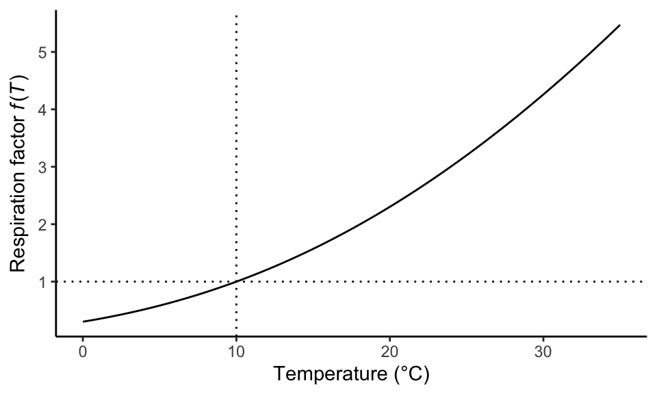
5.1.2 Net primary productivity
At the plant-level, C used for growth is supplied by NSC. The availability of NSC for growth depends on the balance of C assimilation and autotrophic respiration, is influenced by abiotic conditions (temperature, plant desiccation), and varies over the seasons. For example, when leaves are flushed in deciduous plants, the required C is drawn from the NSC pool. Wood is produced not evenly over the seasons, but in a limited period during the growing season which varies strongly between species. Grasses switch from a vegetative growth phase, producing leaves, in the early season to a seed-producing phase later.
The amount of C invested into growth of new biomass in leaves (\(\Delta C_\mathrm{leaves}\)), fine roots (\(\Delta C_\mathrm{roots}\)), and wood (\(\Delta C_\mathrm{wood}\)) plus the production organic compounds released through leaves (volatile organic compounds, \(C_\mathrm{VOC}\)) and roots (exudates, \(C_\mathrm{exu}\)), plus the change in NSC storage (\(\Delta C_\mathrm{NSC}\)) is equal to the gross primary productivity (GPP) minus autotrophic respiration (\(R_a\)). This is the definition of the ecosystem-level vegetation C mass balance. The sum of biomass production in different plant compartments plus \((C_\mathrm{VOC} + C_\mathrm{exu})\) is referred to as the net primary productivity (NPP) and is commonly expressed for annual total fluxes. Over longer (\(\sim\)annual) time scales, the change in NSC storage can be neglected \((\Delta C_\mathrm{NSC} = 0)\) and the following applies: \[ \begin{aligned} \mathrm{NPP} &= \mathrm{GPP} - R_a \\ &= \Delta C_\mathrm{leaves} + \Delta C_\mathrm{roots} + \Delta C_\mathrm{wood} + C_\mathrm{VOC} + C_\mathrm{exu} \end{aligned} \tag{5.2}\] These two terms \(C_\mathrm{VOC}\) and \(C_\mathrm{exu}\) are difficult to measure in the field and tend to be smaller than the other terms. Therefore, the biomass productivity is more commonly quantified from observations. \[ \mathrm{BP} = \Delta C_\mathrm{leaves} + \Delta C_\mathrm{roots} + \Delta C_\mathrm{wood} \tag{5.3}\] Note that there is often some ambiguity in definitions in the literature and ‘NPP’ is often used instead of ‘BP’. BP is expressed as a flux of C per unit square meter (for example gC m-2 yr-1). It measures the amount of biomass C produced per unit ground area and time. NPP is expressed in the same units and additionally includes C produced and released as volatile organic compounds and exudates. These do not contribute to the biomass of the plant itself and are relatively short-lived. However, they are not in the form of oxidized C (as is \(R_a\)) and therefore are counted towards NPP.
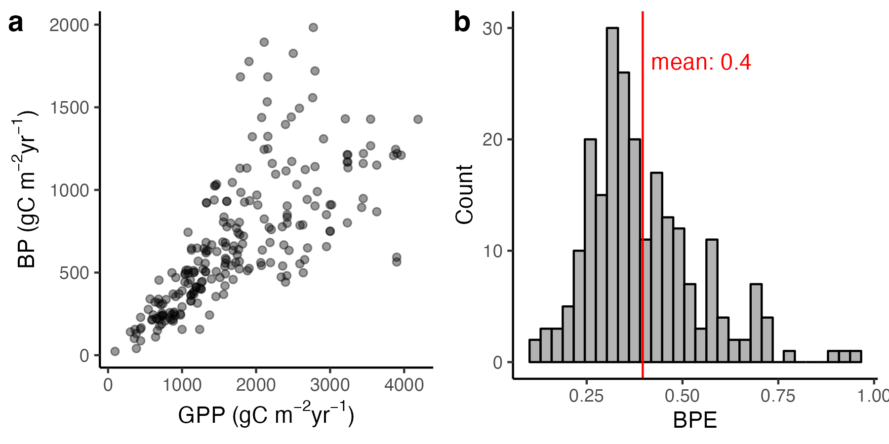
The ratio of NPP:GPP is commonly referred to as the ecosystem carbon use efficiency (CUE), and BP:GPP as the biomass production efficiency (BPE).
\[ \begin{aligned} \mathrm{CUE} &= \mathrm{NPP} / \mathrm{GPP} \\ \mathrm{BPE} &= \mathrm{BP} / \mathrm{GPP} \end{aligned} \tag{5.4}\]
As shown in Figure 5.3, BP is linearly related to GPP across ecosystems, indicating that BP can be assumed to be a constant fraction of GPP - albeit with substantial uncertainty.
CautionExercise
- What is a typical magnitude of \(R_a\), expressed as a fraction of GPP?
5.1.3 Allocation and growth
The partitioning of available NSC to growth in different plant compartments, to VOC, exudates, or respiration is referred to as allocation. Quantitatively, allocation to a given compartment can be expressed as the ratio of BP of that compartment (leaves, roots, wood) over the total NPP. \[ \alpha_i = \Delta C_i / \mathrm{NPP} \tag{5.5}\] Since C allocated to exudates and volatile organic compounds are rarely measured, BP is commonly used instead of NPP in Equation 5.5.

The absence of woody biomass and C allocation to wood production in grasses and herbs as opposed to woody plants (trees and shrubs) is a major difference of allocation across different vegetation types and biomes. While in forests, about half of the total BP is in woody biomass, in grasslands, this is zero. In grasslands, the fractional allocation to leaves and fine roots is about twice as high as in forests (Table 5.1).
| Vegetation | Leaves | Wood | Roots |
|---|---|---|---|
| Forest | 0.28 | 0.47 | 0.27 |
| Grassland | 0.47 | 0.00 | 0.53 |
The fractional belowground C allocation is under a strong influence by environmental conditions (nutrient availability, water availability, and CO2). The fraction of C allocated to fine root growth tends to increase under poor soil nutrient availability, under elevated CO2 (as seen in experiments), and under dry conditions. This can be understood as a response to the balance of above vs. belowground resource availabilities (light and CO2 vs. nutrients and water).
Because C in leaves and fine roots has a much shorter turnover time than in wood, allocation is a key quantity that controls the effective ecosystem C turnover time and ecosystem C dynamics. Thus, a changing environment affects ecosystem C dynamics, i.a., through its influence on allocation.
5.1.4 Biomass turnover and litterfall
Turnover of different plant compartments is driven by different processes. The leaf turnover in grasses and deciduous trees is linked to the seasons. In evergreen trees, the leaf turnover time (or leaf longevity) is commonly longer than one year and is related to the leaf mass per unit leaf area (LMA - thicker leaves live longer). Leaves may also be damaged and shed after severe water stress and exposure to desiccation. Fine roots turn over at time scales of months to years. Woody biomass is much more long-lived than fine roots and leaf biomass. Its turnover is governed by tree mortality (Section 5.4) and ecosystem disturbances (Section 5.5) or the mortality of individual branches of a tree.
5.1.5 Soil and litter C dynamics
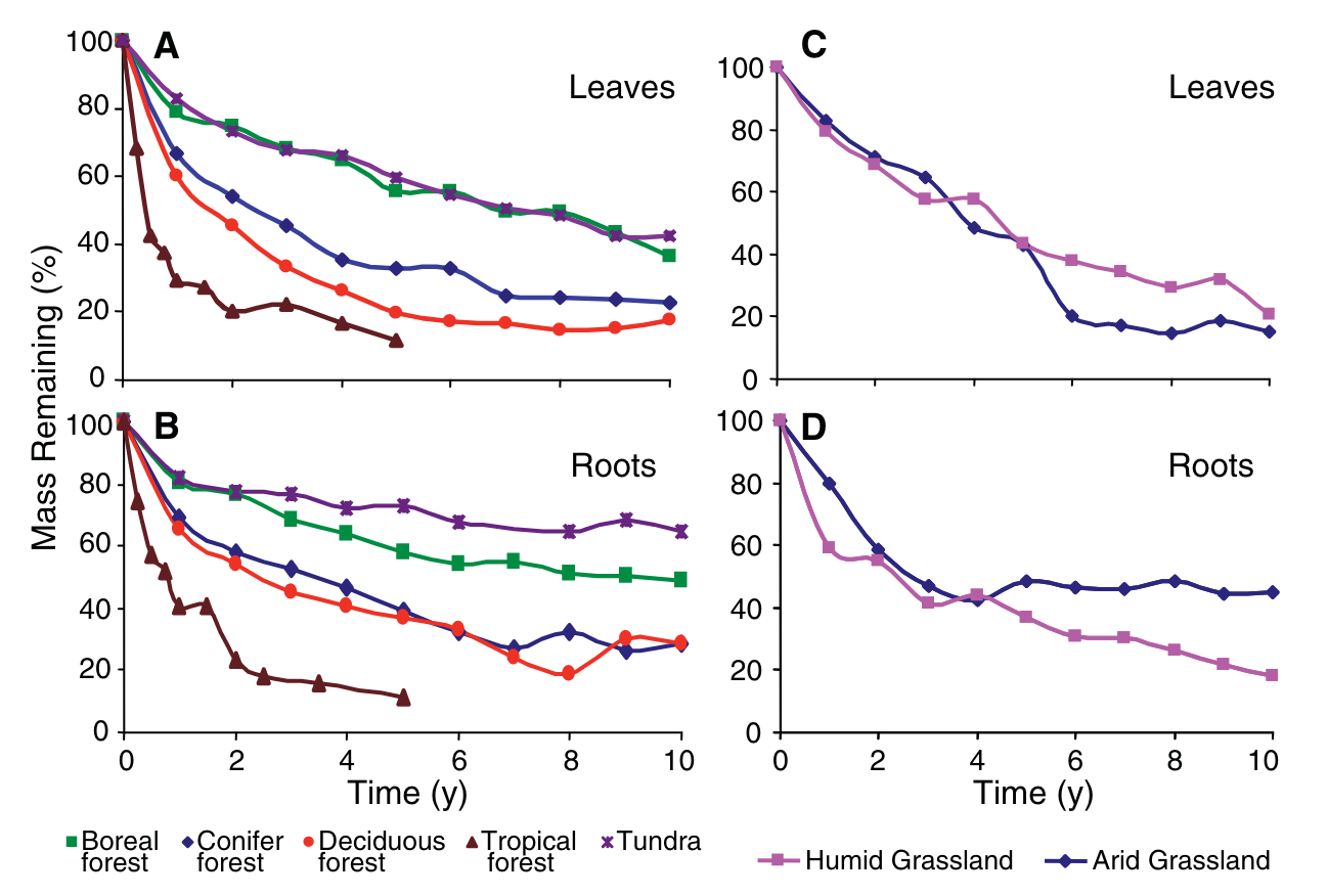
Senesced leaves are shed and, together with deadwood, form the litter pool on the ground surface. Litter is decomposed by soil microorganisms - heterotrophic organisms - that gain energy from consuming the organic matter. Litter also gets mixed into the topsoil by bioturbation (mixing by the soil fauna). C in the litter pool has a turnover time on the order of months to years for the fast-decomposing litter of dead leaves and fine roots (Figure 5.5), to 101-102 years for deadwood. Litter can have an important role as fuel for fire and as an insulation layer between soil and air.
The rate of litter decomposition is strongly affected by temperature and moisture. The warmer, the more rapid the decomposition. The moisture-dependency is a peaked relationship. Below the peak, decomposition increases with moisture. Above the peak, it declines due to a lack of oxygen. The decomposition rate is also influenced by the chemical composition. As a consequence of this environment-dependency, the time scale of litter decomposition varies across biomes (Figure 5.5). Lignified (woody) biomass decomposes more slowly than, e.g., fine roots and leaves.
Soil organic matter (SOM) refers to the organic mass fraction in soils. It consists of litter at advanced stages of decomposition and of microbial biomass and necromass. The decomposition rate of organic matter in soil can be strongly reduced compared to the decomposition rate of litter. This is due to stabilisation processes. Stabilisation of SOM arises from the chemical transformation through soil micro and macro-fauna and through physical protection in the soil matrix (association to minerals, occlusion in soil aggregates). Yet, the decomposition of SOM is rarely fully suppressed (except under fully anoxic conditions).
SOM exposed to decomposition is consumed by microbes (fungi and bacteria) and fuels their growth. As they consume organic matter - like humans - they use the chemical energy “stored” in organic matter and oxidise the carbohydrates to CO2. The CO2 is respired away in gaseous form and leaves the soil volume and is referred to as heterotrophic respiration (\(R_h\)). The rate of microbial activity and hence \(R_h\) increases with temperature in a similar way as the temperature dependency of \(R_a\). \(R_h\) also depends on soil moisture and has a peaked relationship. It initially increases with increasing soil moisture until a point where the oxygen availability in the soil prohibits activity by heterotrophic microorganisms. At this point, \(R_h\) drops sharply. Under water-logged soil conditions, SOM decomposition and \(R_h\) are suppressed. The temperature dependency of \(R_h\), implemented in the LPJ vegetation model is the same as described for \(R_m\) by Equation 5.1.
SOM plays important roles for global biogeochemical cycles and for land-climate interactions. SOM is a vast store of C (~1700 PgC, see Figure 3.1). The soil organic matter content is an important measure for nutrient availability, and strongly influences the water holding capacity of the soil (Chapter 7). C in soil organic matter (SOM) has a turnover time on the order of years to centuries. Under anoxic conditions, the turnover time of SOM can attain millennia. As for litter decomposition, the rate of SOM decomposition (\(k\) in Equation 5.6) is controlled by the soil temperature and moisture.
Note1st-order decay model for litter and SOM
Soil and litter C dynamics can be conceived as a 1-st order decay model, consisting of multiple pools, characterized by distinct turnover rates, and supplied with biomass turnover from different plant compartments. The dynamics of an individual pool can be described following 1st-order dynamics (Box in Section 3.2). \[ \frac{\mathrm{d}C}{\mathrm{d}t} = I - k(T,\theta) \;C \;. \tag{5.6}\] Terrestrial biosphere models commonly treat the decay rate \(k\) as a function of temperature and moisture, as indicated in Equation 5.6 (\(T\) is temperature, \(\theta\) is soil moisture). Some models also use the pH of the soil solution and the oxygen content in the soil for modifying \(k\). \(k\) at a standard temperature varies for different pools, ranging from 1/3-1 years-1 for litter, to 50-500 years-1 for SOM.
Experiments of litter decomposition in the field, where a specified initial mass of litter is tracked over time (Figure 5.5), reveal a general pattern that is consistent with the 1st-order decay model. The solution of Equation 5.6 with \(I=0\) yields: \[ C(t) = C_0\; e^{-k t}\;, \] where \(t\) is time. Indeed, the litter mass shown in Figure 5.5 exhibits an exponential decline over time.
Also SOM decay can be represented following Equation 5.6. In words, the amount of SOM C that gets decomposed in a given amount of time is proportional to the SOM C pool size. The input into that pool is independent of the pool itself.
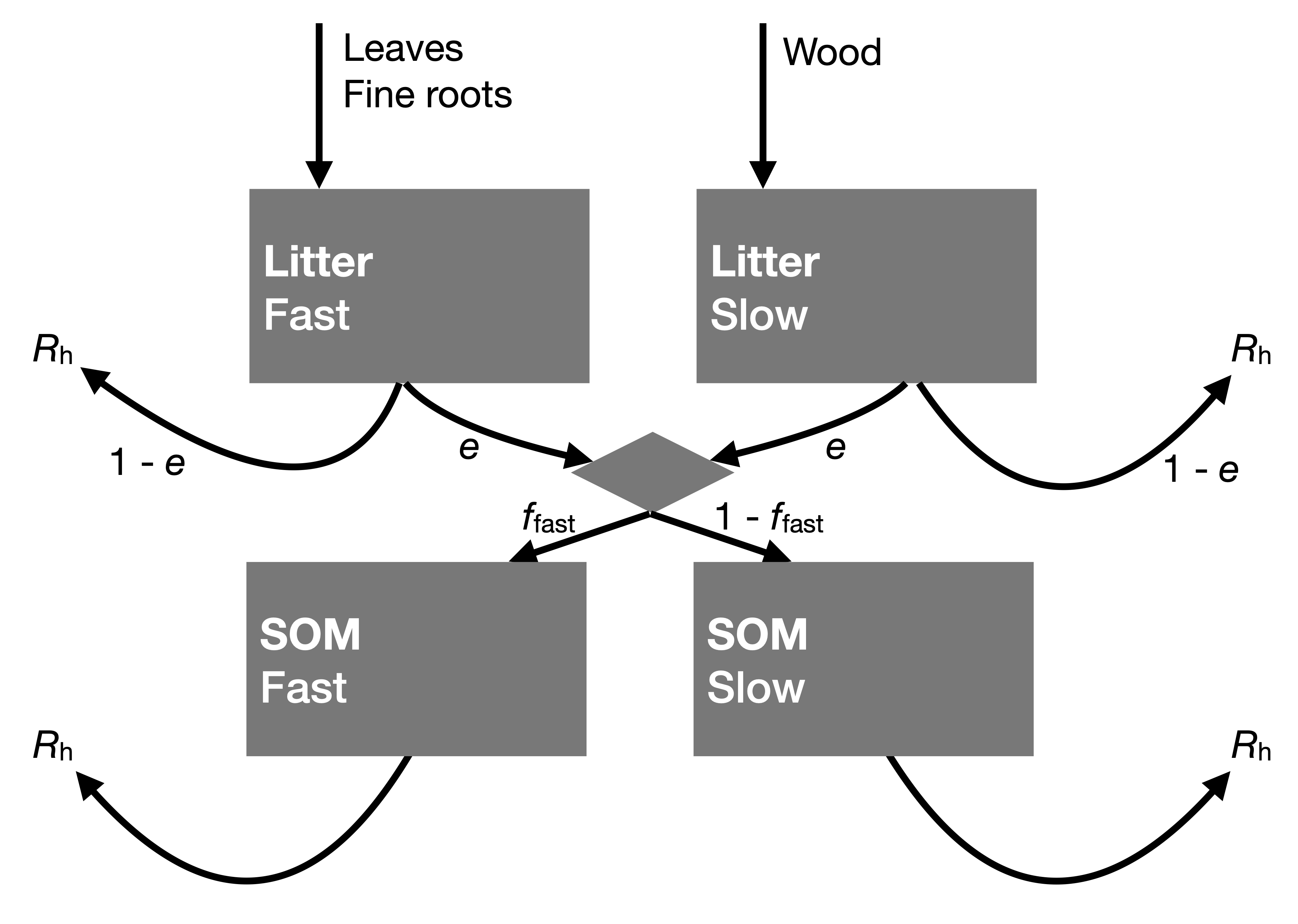
Litter and SOM pools in terrestrial biosphere models are most commonly represented by an array of pools that are characterized by different turnover times and that are connected following a specific structure. The litter pools receive inputs from biomass turnover. Decomposed litter is diverted to SOM pools. Fast-decomposing litter is diverted to a SOM pool with a short turnover time (high \(k\)), slow-decomposing litter is diverted to a SOM pool with a long turnover time. C is respired away as CO2 during litter and SOM decomposition. The microbial carbon use efficiency (\(e\)) determines the ratio of the decomposed C contributing to microbial biomass growth. \((1-e)\) is respired as CO2.
5.1.6 Net ecosystem productivity
The net of gross primary productivity (GPP), autotrophic respiration by plants (\(R_a\)), and heterotrophic microorganisms (\(R_h\)) is referred to as the net ecosystem productivity, NEP. It is expressed in units of a flux of C mass per unit ground area and time, e.g., gC m-2 yr-1. It measures how much C accumulates in an ecosystem in the form of live biomass, litter, and soil (plus VOC and exudates). Since GPP and respiration terms typically have a strong seasonality and diurnal cycle and are not (perfectly) synchronized, NEP has a strong seasonality and diurnal cycle, too (see also Chapter 6). However, integrated over a year, the NEP is small - much smaller than the absolute of its components GPP, \(R_a\), and \(R_h\).
\[ \begin{align} \mathrm{NEP} &= \mathrm{GPP} - R_a - R_h \\ &= \mathrm{NPP} - R_h \end{align} \tag{5.7}\] NEP can be measured by eddy covariance flux measurement technique. The net CO2 exchange (NEE) between the canopy and the atmosphere is measured. It is termed NEE (and not NEP) because the processes and components are not directly identified by the measurement. For example, chemically dissolved C in the soil solution and particulate organic matter may be laterally transported off-site and is not reflected in the measurements. NEE is defined such that negative values indicate a net C gain by the ecosystem - opposite to the definition of NEP.
The classical model of ecological succession and an ecosystem’s carbon balance is that it reaches a steady state at time scales of forest stand maturity (shorter for grasslands), where, under constant environmental conditions, the NEP approaches zero. Respiration balances photosynthetic C uptake, biomass turnover balances biomass accumulation, and ecosystems become “C neutral” (Odum 1969).
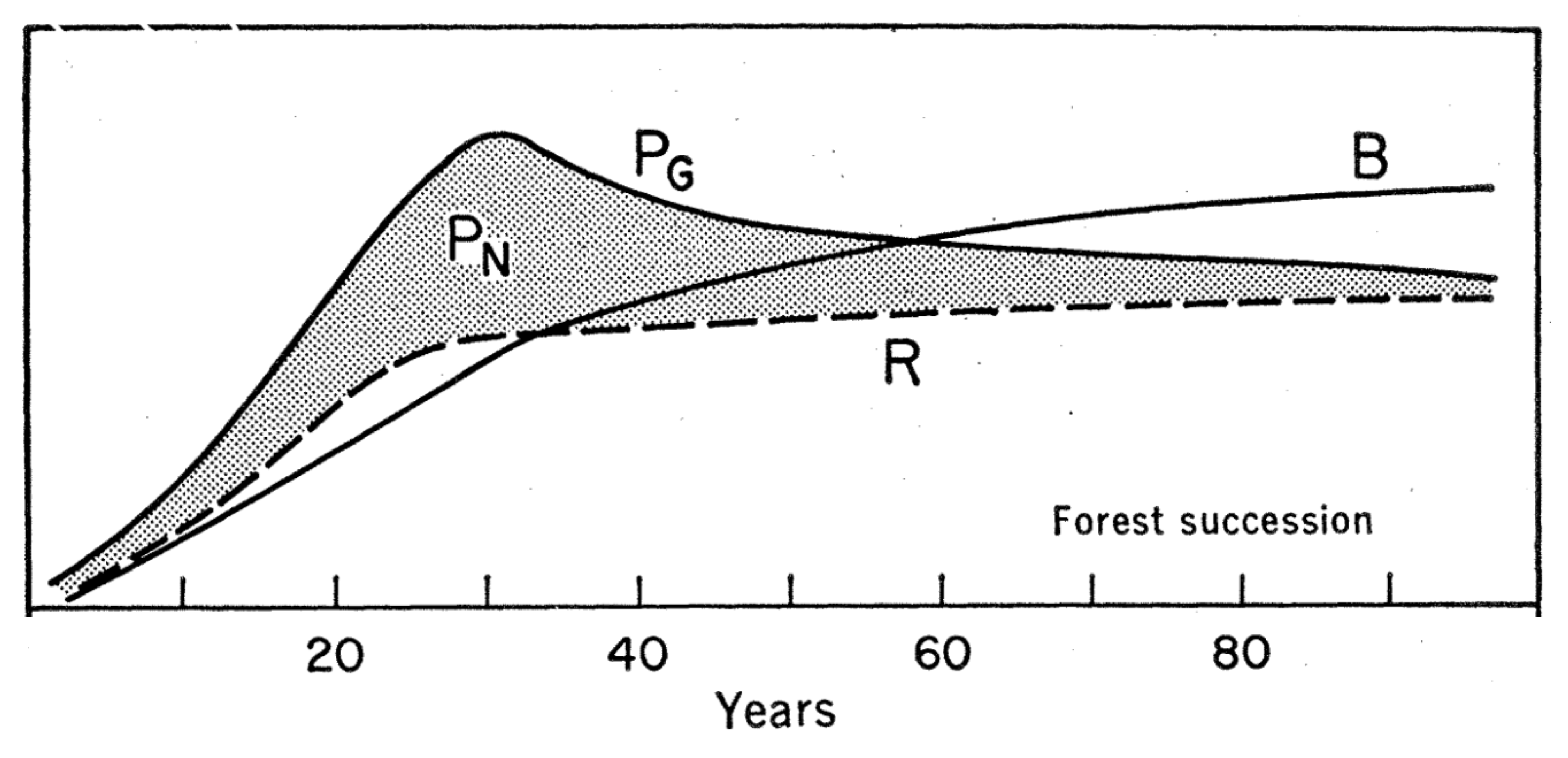
However, field data of biomass stocks in mature forests seem to contradict Odum’s steady state (and zero NEP) model (Luyssaert et al. 2008). Biometric data (forest inventories) and eddy covariance flux measurements from forests do not show a clear decline of NEP towards zero with increasing stand age, but rather show a sustained positive NEP over several decades to centuries since forest stand development.
Will forests accumulate C indefinitely? Tracking soil C stocks over millennia is per se not possible but clear patterns of a positive influence of soil age on SOM content would have to be evident in data - but are not. Biomass C stocks do not increase indefinitely, either. Individual trees in maturing forest stands continue accumulating biomass but the lifetime of a tree is limited due to hydraulic, mechanical, or C balance constraints whereby increasing respiratory costs pose limits to further growth and may trigger mortality. Self-thinning drives the exclusion of individual trees based on the competition for limited resources and leads to a negative relationship between the number and the average size of trees in a maturing forest stand (see Section 5.4). Therefore, although individual trees may accumulate C in the form of biomass for centuries, the biomass C accumulation at the stand level is much lower due to the declining tree number and the associated mortality, turnover, and decomposition of affected trees.
Very old stands are dominated by few very large individual trees that contribute strongly to the total ecosystem biomass. However, also these individuals are inevitably affected by mortality. Once they fall, the ecosystem C stock rapidly declines (NEP is negative) and they create a forest gap that enables younger and smaller individuals to benefit from increased light levels. Smaller individuals around the newly formed gap accelerate growth, reach the canopy, and eventually fill the gap.
These dynamics imply that the NEP is rarely zero, but is positive for most of the time, except when affected by rare mortality events of large individuals. The spatial extent of a forest gap is on the order of 100-101 m and the maximum tree longevity is on the centuries (and the probability of a tree dying in a given year is its inverse - on the order of 10-2). This implies that the probability of observing a gap formation within a given areal extent is a function of the size of the areal extent. The larger the areal extent, the larger the probability that the influence of gap formation on NEP is captured and the large negative NEP of the gap is balanced by the small positive NEP of the remaining forest area. With an increasing size of the areal extent, the mean NEP should therefore tend to zero.
Forest monitoring plots are usually on the order of 20-50 m in radius. Hence, such data is sensitive to whether the observed plots are a representative sample of forest dynamics and forest gap formation across the landscape.
5.1.7 Net biome productivity
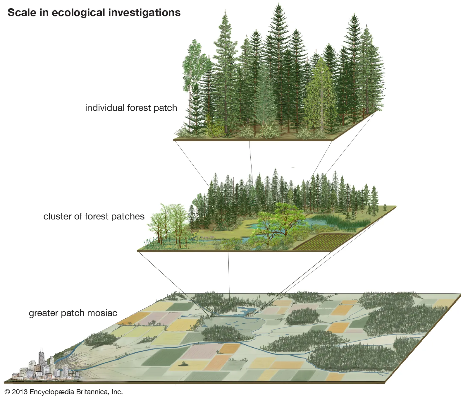
Net biome productivity (NBP, expressed in a mass carbon per unit ground area and time, for example gC m-2 yr-1) is the net of NEP and C loss by disturbances \(\Delta C_\mathrm{dist}\). The NBP is defined for large spatial domains - large enough to contain a representative sample of stochastically occurring disturbances. Across an entire biome, this is given. \[ \begin{align} \mathrm{NBP} &= \mathrm{GPP} - R_a - R_h - \Delta C_\mathrm{dist} \\ &= \mathrm{NEP} - \Delta C_\mathrm{dist} \end{align} \tag{5.8}\] Disturbances are commonly referred to as stand-replacing events that drive mortality in a large portion of individual plants of an ecosystem. Causes for disturbances include fire, pests, windthrow, or wood harvesting. A disturbance can be conceived as a re-setting of the “Odum-type” ecosystem succession. In contrast to the forest gap dynamics (Section 5.1.6), which play out at the level of individual trees, disturbances affect larger spatial extents (ecosystem or forest patches, Figure 5.8). However, the same aspects of stochasticity across the landscape applies.
At the landscape-level, a forest can be conceived as a mosaic of forest patches, characterized by different times since the last stand-replacing disturbance. The first years after a disturbance, ecosystems tend to lose C (negative NEP). This is because the respiration from decomposing litter outweighs the biomass production of regrowth. After a few years, this balance reverses and the ecosystem total C stock increases. Although individual patches tend to have a positive NEP, a small portion of young patches will have a strongly negative NEP. When considering a large number of patches in absence of environmental change (driving trends in GPP, \(R_a\), \(R_h\) or the disturbance probability), the mean NEP across patches - this is the NBP - tends to zero.
The terrestrial carbon balance can be understood of the global total NBP.
5.2 The C cascade model
The C cascade model (Figure 5.9) integrates the information about ecosystem carbon pools and fluxes, provided above in this Chapter. A key insight is that C only enters ecosystems through photosynthesis, measured at the ecosystem-level by GPP. Once in the system, it fuels a “cascade” of pools. They can be conceived as a cascade because biomass pools receive C inputs only through GPP (minus \(R_a\)), litter pools only receive C inputs through biomass turnover, and SOM pools only receive C inputs through litter decomposition. Along this cascade, autotrophic and heterotrophic respiration incurs an ecosystem C loss. The rate at which C cascades through this system depends on the turnover rates of the individual pools and on the relative partitioning (allocation and partitioning to different litter and SOM pools) into the “downstream” pools. A schematic of the C cascade can be drawn by extending Figure 5.6.
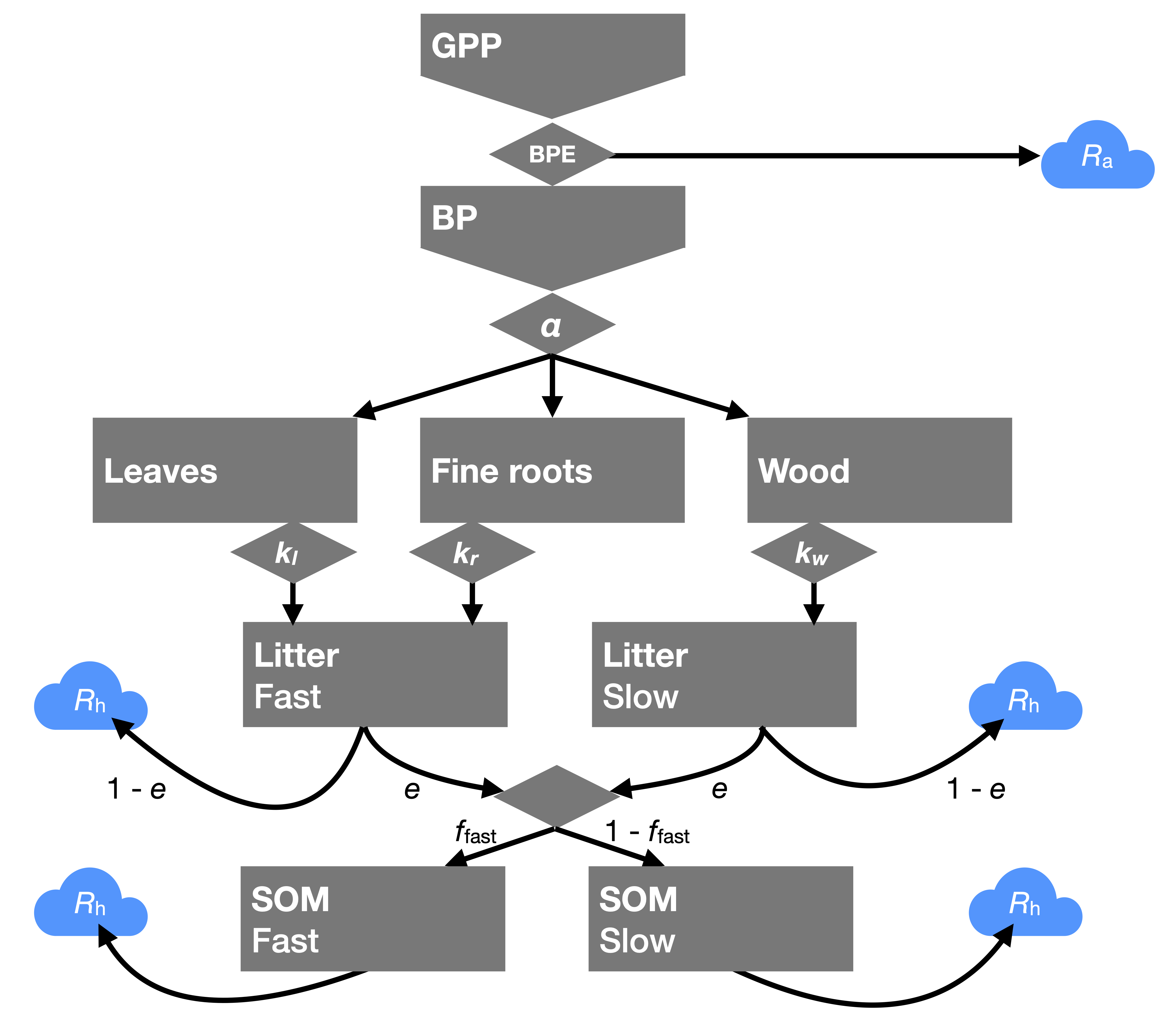
Figure 5.9 illustrates the pivotal role of BPE in determining how much C enters more long-lived storage as biomass vs. its largely immediate loss through respiration, of allocation in diverting C streams along cascades of very different turnover times (e.g., leaf vs. wood allocation), of microbial carbon use efficiency, and of processes determining the partitioning of C into (protected) slowly decomposing SOM pools and more rapidly decomposing SOM pools.
In Chapter 3, we simulated the response of terrestrial C storage to an increased GPP using a 1-box model and 1st-order decay. In this Chapter, we have “unboxed” C storage in terrestrial ecosystems, distinguishing a suite of pools and fluxes, arranged in a cascading order. When considering the response of this system to a change in GPP, how does the more complex representation affect the dynamics?
A key characteristic of the 1st order decay model is that the steady-state C pool size \(C^\ast\) is proportional to (is linearly dependent on) the input flux (Equation 3.4). Hence, with a change in the input flux of \(x = I/I_0\), the steady-state pools size changes also by \(x = C^\ast/C^\ast_0\).
It can be demonstrated (see Box ‘Simulating the C cascade’ below) that when considering the following properties for the C cascade model:
- 1st-order decay dynamics of all pools
- constant \(\alpha\), \(k_i\), \(e\), and \(f_\mathrm{fast}\)
…, the same linear dependency of the total system C storage \(\sum_i C_i^\ast\) emerges: \[ \frac{I}{I_0} = \frac{\sum_i C_i^\ast}{\sum_i C_{i,0}^\ast} = \frac{C_i^\ast}{C_{i,0}^\ast}, \; \forall i \] The symbol \(\forall\) means ‘for all’. However, whether a model with constant \(\alpha\), \(k_i\), \(e\), and \(f_\mathrm{fast}\) is a good representation of real ecosystems’ responses to environmental change is questionable. It is well established, for example, that \(\alpha\) is very sensitive to altered soil nutrient availability and changes in CO2 experiments (Poorter et al. 2012). The turnover rate of biomass in forests (or tree longevity) may be affected by accelerated self-thinning if environmental change positively influences tree-level growth (e.g., through CO2 fertilization or an extension of the growing season) (Marqués et al. 2023). This implies a departure from the linear systems behavior of the C cascade model described by the two points above.
TipSimulating the C cascade
The two points (see above) are implemented in a multi-box model:
- 1st-order decay dynamics of all pools
- constant \(\alpha\), \(k_i\), \(e\), and \(f_\mathrm{fast}\)
The following parameters are set:
Code
library(dplyr)
source(here::here("R/ccascade.R"))
getpar() |>
  as_tibble() |>
knitr::kable()| bpe | fleaf | froot | fwood | kleaf | kwood | kroot | kflitt | kslitt | kfsoil | kssoil | eff | ffast |
|---|---|---|---|---|---|---|---|---|---|---|---|---|
| 0.4 | 0.3 | 3 | 0.4 | 0.5 | 0.02 | 0.5 | 0.5 | 0.1 | 0.1 | 0.003 | 0.6 | 0.95 |
The model is “spun-up” to a steady state for 3000 simulation years. The turnover time of the slowest pool (here the slow soil pool, kssoil = 0.003, corresponding to 333 years) is indicative of how long the model has to be spun-up.
The GPP is then increased from 100 PgC yr-1 during the first 3000 simulation years to 120 PgC yr-1 for the subsequent 3000 simulation years.
Code
# specify GPP for each simulation year as a vector
gpp <- c(rep(100, 3000), rep(120, 3000))

# run the model, it returns a data frame
df <- ccascade(gpp)

library(ggplot2)
df |>
  ggplot() +
  geom_line(aes(year, cleaf, color = "Leaf C")) +
  geom_line(aes(year, cwood, color = "Wood C")) +
  geom_line(aes(year, croot, color = "Root C")) +
  geom_line(aes(year, flitt, color = "Fast litter C")) +
  geom_line(aes(year, slitt, color = "Slow litter C")) +
  geom_line(aes(year, fsoil, color = "Fast soil C")) +
  geom_line(aes(year, ssoil, color = "Slow soil C")) +
  geom_vline(xintercept = 2500, linetype = "dotted") +
  geom_vline(xintercept = 5500, linetype = "dotted") +
  xlim(2000, 6000) +
  khroma::scale_color_okabeito(name = "") +
  theme_classic() +
  labs(x = "Simulation year", y = "Pool size (PgC)")
The relative change in each pool can be quantified by comparing the pool sizes, e.g., in simulation year 2500, with the pool sizes in simulation year 5500.
Code
library(tidyr)
df_plot <- df |>
  filter(year == 2500) |>
  pivot_longer(2:10, names_to = "variable", values_to = "value_2500") |>
  select(-year) |>
  left_join(
    df |>
      filter(year == 5500) |>
      pivot_longer(2:10, names_to = "variable", values_to = "value_5500") |>
      select(-year),
    by = "variable"
  ) |>
  mutate(rel_change = value_5500 / value_2500)

df_plot |>
  filter(!(variable %in% c("ra", "rh"))) |>
  ggplot(aes(value_2500, value_5500, color = variable)) +
  geom_abline(slope = 1, linetype = "dotted") +
  geom_abline(slope = 1.2, color = "grey") +
  geom_point(size = 3) +
  khroma::scale_color_okabeito(name = "") +
  theme_classic() +
  labs(x = "Pool size in year 2500 (PgC)",
       y = "Pool size in year 5500 (PgC)")
This illustrates that the relative change in the size of each pool in the C cascade is identical and corresponds to the relative change in GPP. In other words, the C cascade with constant allocation, turnover rates, and efficiencies exhibits a linear systems dynamics.
NoteWhat is the C balance effect of planting a forest?
Planting a forest on land that was previously a grassland, if well attended to and not affected by disturbances (e.g., drought-induced tree mortality, pests, or fire), may lead an increase in the biomass C stock over the course of several decades. Ignoring effects on the soil C stock, this implies that planting a forest sequesters C.
How does this relate to the C cascade description of ecosystem C dynamics in this chapter? A notable aspect is that photosynthesis rates and GPP are similar in grasslands and forests. If the same amount of C enters the ecosystem, why is the C storage larger in a forest than in a grassland?
Of course, C in woody biomass has a much longer turnover time than C in leaves and fine roots. Therefore, following the logic of the box modelling and 1st-order decay, the steady-state C stock in biomass is larger in a forest than in a grassland despite GPP being similar.
How effective are forest plantations for compensating CO2 emissions? Again, let’s turn to the box model. We may assume that GPP is 1500 gC m-2 yr-1 and that a forest is planted in simulation year 10 - implemented in the model by increasing the allocation fraction to wood from zero initially (in a grassland) to 0.5 from year 10 onwards. The turnover time of leaves and fine roots is 2 years and 50 years for woody biomass.
The model simulation below shows the accumulation of vegetation biomass (leaf, root, and wood C) over time and the net ecosystem productivity - measuring the C balance of the ecosystem.
Code
library(dplyr)
library(ggplot2)
library(cowplot)
source(here::here("R/ccascade.R"))

# first spin up the C cascade model representing a grassland
# modify default parameters for allocation
par <- getpar()
par$fwood <- 0
par$fleaf <- 0.5
par$froot <- 0.5

# specify GPP (gC m-2 yr-1) for each simulation year as a vector
gpp <- rep(1500, 3000)

# run the model, it returns a data frame
df_spinup <- ccascade(gpp, par = par)

# save state and fluxes after spinup
state <- df_spinup |>
  tail(1) |>
  select(cleaf, cwood, croot, flitt, slitt, fsoil, ssoil) |>
  as.list()

fluxes <- df_spinup |>
  tail(1) |>
  select(ra, rh) |>
  as.list()

# run model forward (300 years), converting to forest in year 10 (changing allocation)
# GPP as forcing
gpp <- rep(1500, 300)

len <- length(gpp)

# output the state and fluxes in one data frame
df <- dplyr::tibble()

# integrate over each time step (this is an implementation of the differential equation)
for (yr in seq(len)){

  if (yr == 10){
    par$fwood <- 0.5
    par$fleaf <- 0.3
    par$froot <- 0.2
  }

  # update states and fluxes
  out <- ccascade_onestep(
    gpp[yr],
    state,
    par,
    fluxes
    )

  state <- out$state
  fluxes <- out$fluxes

  # record for output
  df <- dplyr::bind_rows(
    df,
    dplyr::bind_cols(
      dplyr::tibble(year = yr),
      dplyr::as_tibble(state),
      dplyr::as_tibble(fluxes))
    )
}


gg1 <- df |>
  ggplot() +
  geom_line(aes(year, (cleaf + cwood + croot)/1000)) +
  geom_vline(xintercept = 10, linetype = "dotted") +
  theme_classic() +
  labs(
    x = "Simulation year",
    y = expression(paste("Biomass C (kgC m"^-2, ")"))
    )

gg2 <- df |>
  mutate(nep = gpp - ra - rh) |>
  ggplot() +
  geom_line(aes(year, nep)) +
  geom_vline(xintercept = 10, linetype = "dotted") +
  theme_classic() +
  labs(
    x = "Simulation year",
    y = expression(paste("NEP (gC m"^-2, "yr"^-1, ")"))
    )

plot_grid(gg1, gg2, ncol = 1)
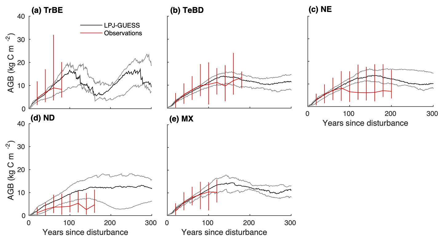
This illustrates that a forest is only a net C sink during its establishment. Once a new steady state is reached, biomass C no longer increases and NEP declines to zero. Forest plantations do not provide sustained CO2 removal. A mature forests tends towards becoming “C-neutral”.
Observations-based forest biomass regrowth curves, and curves simulated by a Dynamic Global Vegetation Model (DGVM) for different biomes are shown in Figure 5.14.
CautionExercise
- Which pool in the C cascade model (Figure 5.9) has the slowest C turnover? What is its turnover time \(\tau\), considering model parameter values given in Figure 5.10?
- Consider the visualisation of litter decomposition in different biomes (Figure 5.5), and the 1st-order decay model. Establish the order of each biome’s decay constant \(k\) (e.g., \(k_\mathrm{biome1} < k_\mathrm{biome2} < ...\)).
- Consider two ecosystems (\(a, b\)) that differ with respect to their photosynthetic rates (\(\mathrm{GPP}_a < \mathrm{GPP}_b\)), but have identical (constant) carbon pool turnover times \(k_i\), identical (constant) allocation fractions \(\alpha\), and identical (constant) soil organic matter dynamics (identical \(f_\mathrm{fast}\) in the C cascade model). Which of the two has a higher steady-state total ecosystem C storage, considering the C cascade model and 1-st order decay in each C pool?
- Consider the same setup as in (3.), but now you have more information about the relative magnitudes of \(\mathrm{GPP}_a\) and \(\mathrm{GPP}_b\): \[ \mathrm{GPP}_b / \mathrm{GPP}_a = 1.2 \] What is the ratio of steady-state ecosystem C storage in the two ecosystems?
- Discuss whether the C cascade model and the result obtained for (4.) is an accurate model for the real world. Do you expect the ratio of steady-state C storage in response to a 20% increase in GPP to be higher or lower than 20%? Do you expect BPE, allocation fractions \(\alpha_i\), and decay constants \(k_i\) to change in response to increases in GPP?
- What quantity do you consider for measuring the annual C balance of an ecosystem? 7, What quantity do you consider for measuring the annual C balance of forests, grasslands, and agricultural lands in Switzerland?
5.3 Tree growth and allometry
Coming soon.
5.4 Forest dynamics
Coming soon.
5.5 Fire and other disturbances
Coming soon.