8 Ecohydrology
8.1 Global water cycle
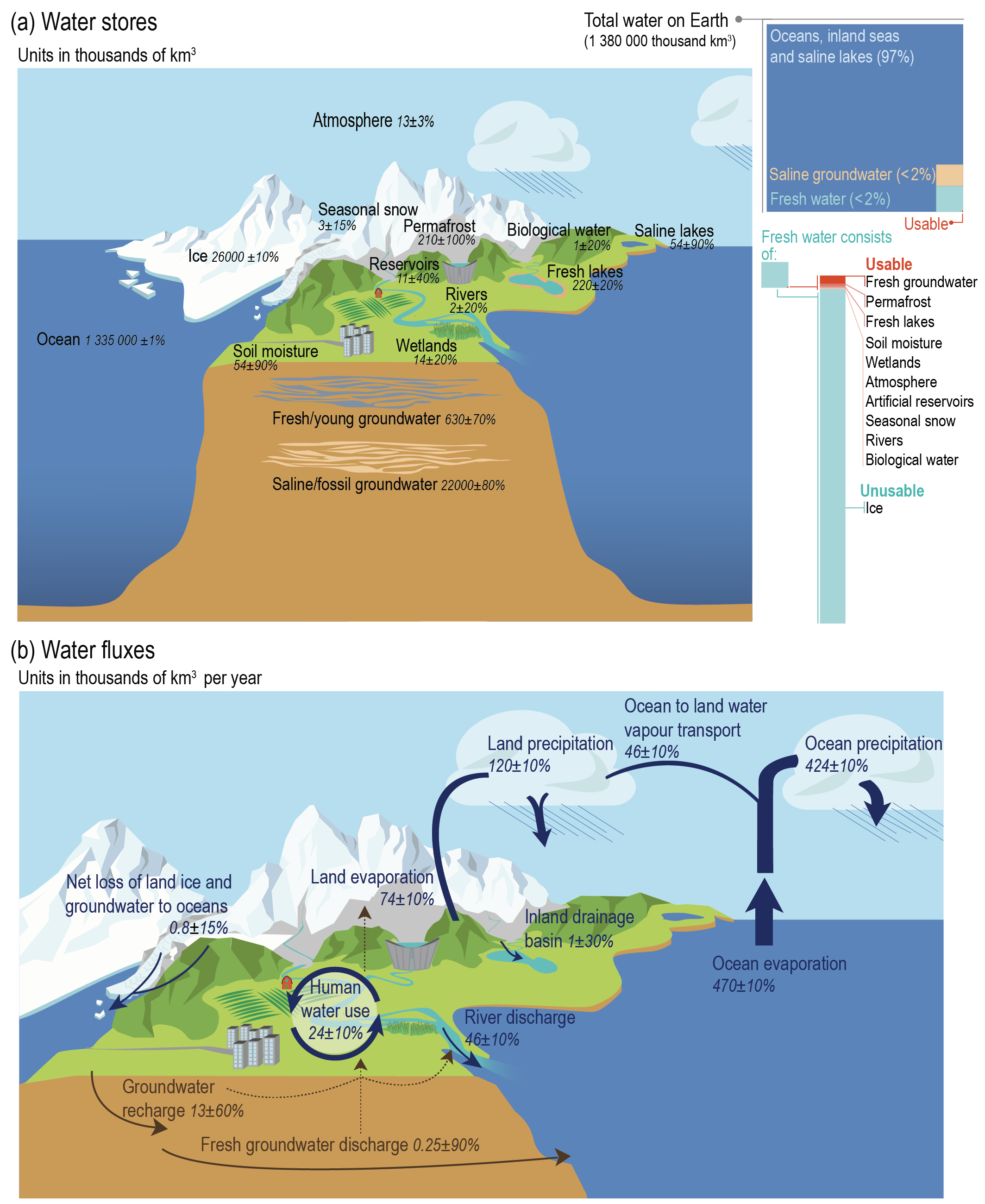
Water cycles in the Earth system between the atmosphere, the ocean, the land biosphere and the cryosphere. The evaporation of water (H2O) from its liquid form to (gaseous) water vapor consumes energy (Section 7.2) and its condensation releases the same amount of energy in the form of heat again. Hence, the global water cycle is coupled to large energy transfers. For the Earth as a whole and as an annual average, 80 W m–2 are consumed for evaporation – more than three-quarters of the 98 W m–2 net radiation at the surface (Bonan 2015).
The vast majority (ca. 98%) of water on Earth is saline and is stored in the Oceans, inland seas, and saline groundwater (Figure 8.1 a). Among the total amount of freshwater, the vast majority is stored as ice. Only a small fraction of water on Earth cycles between the atmosphere, the ocean and land. However, this cycling is relatively rapid (see Exercise below).
Oceans dominate in total evaporation (470 km3 yr-1, vs. 74 km3 yr-1 from land, Figure 8.1 b) and the majority of precipitation falls over oceans. However, since precipitation over oceans is smaller than evaporation from oceans (424 km3 yr-1 vs. 470 km3 yr-1), a net transfer of water from oceans to land exists. Almost all the surplus of the land’s water balance runs off as river discharge back into the ocean. A small fraction is discharged into the ocean through groundwater.

Evaporation from land is a smaller component than evaporation from oceans, and soils store less than 1% of the unfrozen freshwater on Earth. Yet, land processes are a key regulator of global water cycling and energy fluxes. This is because the majority of evaporation over land occurs through transpiration and is thus affected by the vegetation structure and ecophysiological relations - through effects of LAI (Section 4.2), surface conductance (Section 7.2.2) and stomatal conductance (Section 4.4). Another aspect is the fact that, while the amount of water stored in the rooting zone of vegetation is small, it supplies all transpiration. In many climates, the root zone moisture gets substantially depleted during episodic dry spells or regularly recurring dry seasons. The ensuing plant water stress leads to a reduction of transpiration and evaporation, and thus to an alteration also of the surface energy partitioning. This chapter introduces the quantities and mechanisms for understanding how water regulates vegetation and how vegetation shapes the cycling of water and land surface energy partitioning across the globe.
- Calculate the total freshwater stored as ice as a fraction of total freshwater.
- Calculate the turnover time of water in the atmosphere.
- Calculate the turnover time of water in soils (soil moisture).
We have encountered the vapor pressure deficit (VPD) and its control on transpiration in Section 4.4 and on evapotranspiration in Section 7.2.2. VPD is a measure of atmospheric humidity. This box is to explain how VPD relates to other metrics of atmospheric humidity and to the physics of moist air.
The total pressure of a gas can be expressed as the sum of partial pressures of different components of a gas mixture. For moist air, we can distinguish the partial pressures of water vapor (\(e_a\)) and dry air (\(P_d\)) and write the total pressure of moist air as \[ P = P_d + e_a \;. \] Both, the dry air and water vapor follow the ideal gas law. Expressed in molar form, they are \[ P_d = \rho_d \frac{RT}{M_d} \\ \text{ and } \\ e_a = \rho_v \frac{RT}{M_v} = \rho_v \frac{RT}{0.622 M_d} \tag{8.1}\]
Here, \(\rho_d\) is the density of dry air; \(\rho_v\) is the density of water vapor, \(R\) is the universal gas constant (8.314 J K-1 mol-1); \(T\) is temperature (in K). The factor 0.622 relates the molecular mass of water (\(M_v = 18.02\) g mol–1) to that of dry air (\(M_d = 28.97\) g mol–1).
The specific humidity \(q\) can be derived from Equation 8.1 as \[ q = \frac{\rho_v}{\rho_v + \rho_d} = \frac{0.622 e_a}{P-(1-0.622)e_a} \] The vapor pressure deficit (\(D\)) is the difference between the actual vapor pressure \(e_a\) and the vapor pressure at saturation \(e_s(T)\) (where water condensates). \[ D = e_s - e_a \] The saturation vapor pressure is a function of air temperature (\(T\) in °C). This relationship is related to the Clausius-Clapeyron relation of the temperature dependence of vapor pressure. A relatively accurate, yet simple empirical equation for this relationship is the following. \[ e_s(T) = 611.0 \; \exp \left( \frac{17.27 \; T}{T + 237.3} \right) \] This equation calculates the the saturation vapor pressure \(e_s(T)\) in units of Pa.
Code
library(ggplot2)

calc_e_sat <- function(temp){
  611.0 * exp( (17.27 * temp)/(temp + 237.3) )
}

ggplot() +
  geom_function(fun = calc_e_sat) +
  xlim(0, 35) +
  labs(x = "Temperature (°C)",
       y = "Saturation vapor pressure (Pa)") +
  theme_classic()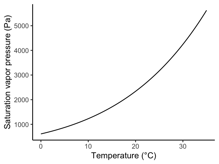
The relative humidity (RH) also relates \(e_a\) to \(e_s\), but as its ratio and not the difference. \[ \mathrm{RH} = 100 \% \; \frac{e_a}{e_s(T)} \]
8.2 Ecosystem water balance
From the conservation of water mass, it follows that the amount of water inputs into an ecosystem through precipitation must equal its outputs plus a change in ecosystem water storage. Outputs are either evaporation or runoff. The ecosystem water balance can thus be expressed as \[ P = E + R + \Delta S \;, \tag{8.2}\] where \(P\) is precipitation, \(E\) is evaporation, which includes different contributions (see below), \(R\) is runoff, and \(\Delta S\) is the change in water storage, mostly in the form of groundwater. Lateral subsurface flow is accounted for by \(R\). Equation 8.2 applies to any system and scale. When considering totals or means of these fluxes over longer periods of time, \(\Delta S\) tends to be small and may be neglected. At the scale of a river catchment, \(R\) is always zero or positive. At smaller scales, horizontal subsurface water flow convergence could make \(R\) negative (“run-on” instead of run-off). \(E\) is the same quantity as the \(E\) in Equation 7.5, but here expressed as a mass flux. (Remember, \(\lambda E\) is the latent heat flux expressed in energy units).
Most commonly, the components of Equation 8.2 are expressed as a mass per unit ground area and time. That is, for example in kg m-2 yr-1. With the density of water \(\rho_w = 1000\) kg m-3, 1 kg m-2 is equivalent to 1 mm.
With \(R \geq 0\) and \(\Delta S = 0\), it follows that \(P \geq E\). On a global average over land, \(E/P = 0.65\). However, \(E/P\) varies between about 0.2 and 1 across different ecosystems, catchments, and biomes. The pattern of how this ratio varies across the globe is described and explained in Section 8.7.
\(E\) in Equation 8.2 includes contributions from multiples sources and processes (Figure 8.3). Below, we will refer to it as evapotranspiration, or short, ET. ET is the sum of transpiration by leaves (\(T\), corresponding to what is referred to as \(E\) in Section 4.4), evaporation from soil (\(E_S\)), evaporation from intercepted water on leaf and branch surfaces (\(E_I\)), and sublimation (\(S\), the phase change from solid water in the form of snow and ice directly to the gaseous phase). \[ E = T + E_S + E_I + S \tag{8.3}\]
The water balance of the rooting zone has to account for the fact that a portion of precipitation is intercepted and evaporates again as \(E_I\). Only the remainder reaches the ground as throughfall. Infiltration is referred to as the moisture flux that reaches a certain depth in the soil. On annual and longer time scales, snow water mass does not accumulate and snow melt equals the amount of precipitation that falls as snow minus sublimation (\(S\)). Snow accumulation and melt is therefore not reflected in Equation 8.2. However, at sub-seasonal time scales, snow accumulation and melting can substantially affect the water root zone water balance (see below).
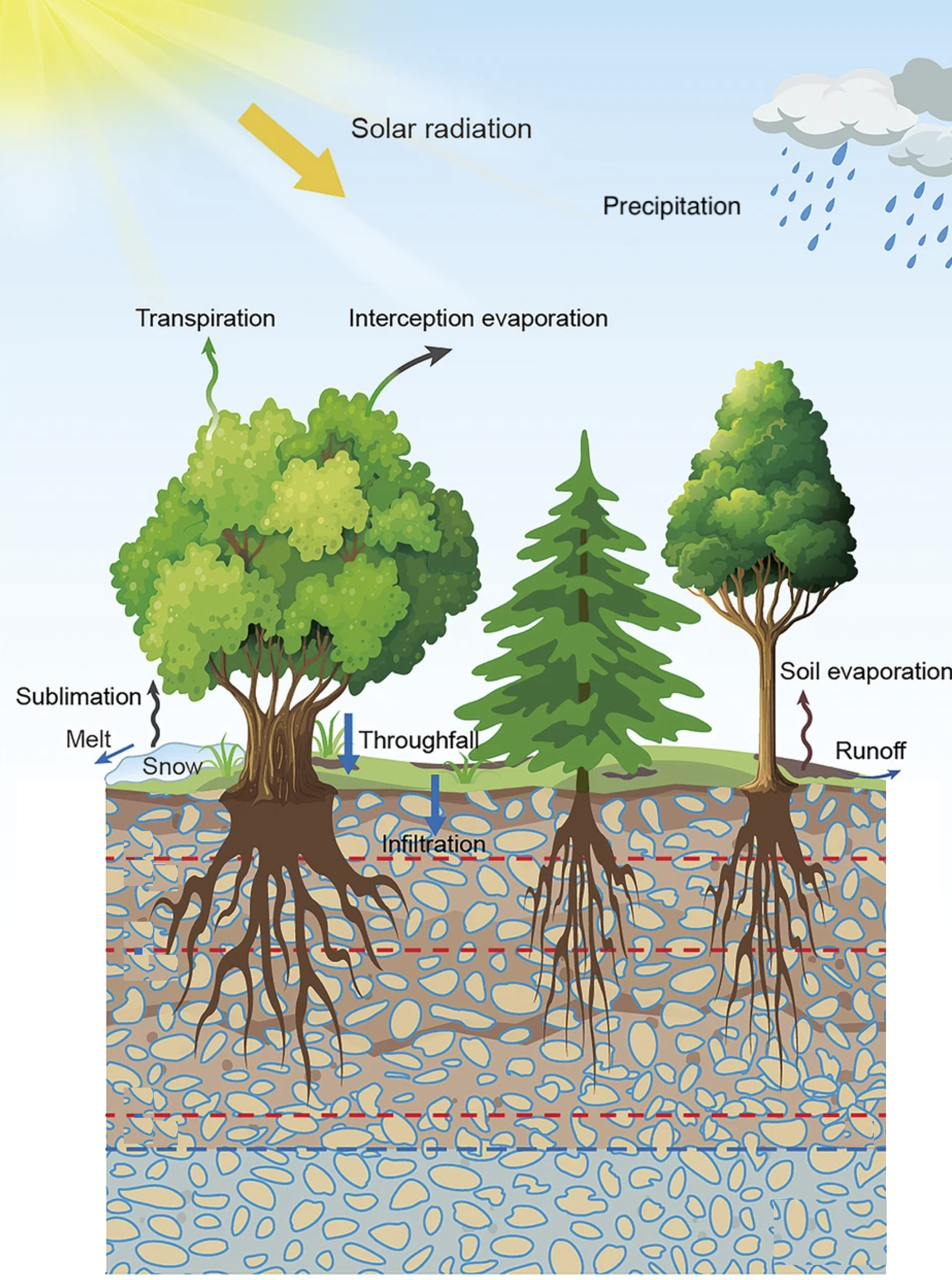
The relative contributions of the different components of ET in Equation 8.3 are difficult to estimate. Model-based estimates for global averages are 48% for transpiration, 36% for soil evaporation, and 16% for canopy evaporation (Dirmeyer et al. 2006). A more recent estimate suggests a higher contribution by \(T\) (Wei et al. 2017). The partitioning depends on ecosystem characteristics, primarily LAI. A high LAI is associated with high \(T\) and \(E_I\). The higher LAI, the lower the radiation reaching the soil surface (Section 4.2) and thus the lower \(E_S\) (noting that energy is required for driving evaporation).
The different components to ET draw water from separate stores - from moisture in the root zone of vegetation for \(T\), from moisture in the top few centimeters of soil for \(E_S\), and from moisture adsorbed on canopy surfaces. Therefore, their evolution over time during dry (rain-free) phases is very different. While \(E_I\) drops to zero within 1-3 days as canopy surfaces become dry, \(E_S\) declines more slowly since the top soil takes longer to dry out to a degree where \(E_S\) becomes zero. In contrast, \(T\) takes much longer to decline as plants may draw moisture from much larger belowground stores - from water stored in the soil and sub-soil across the entire rooting zone.
8.2.1 Cumulative water deficits
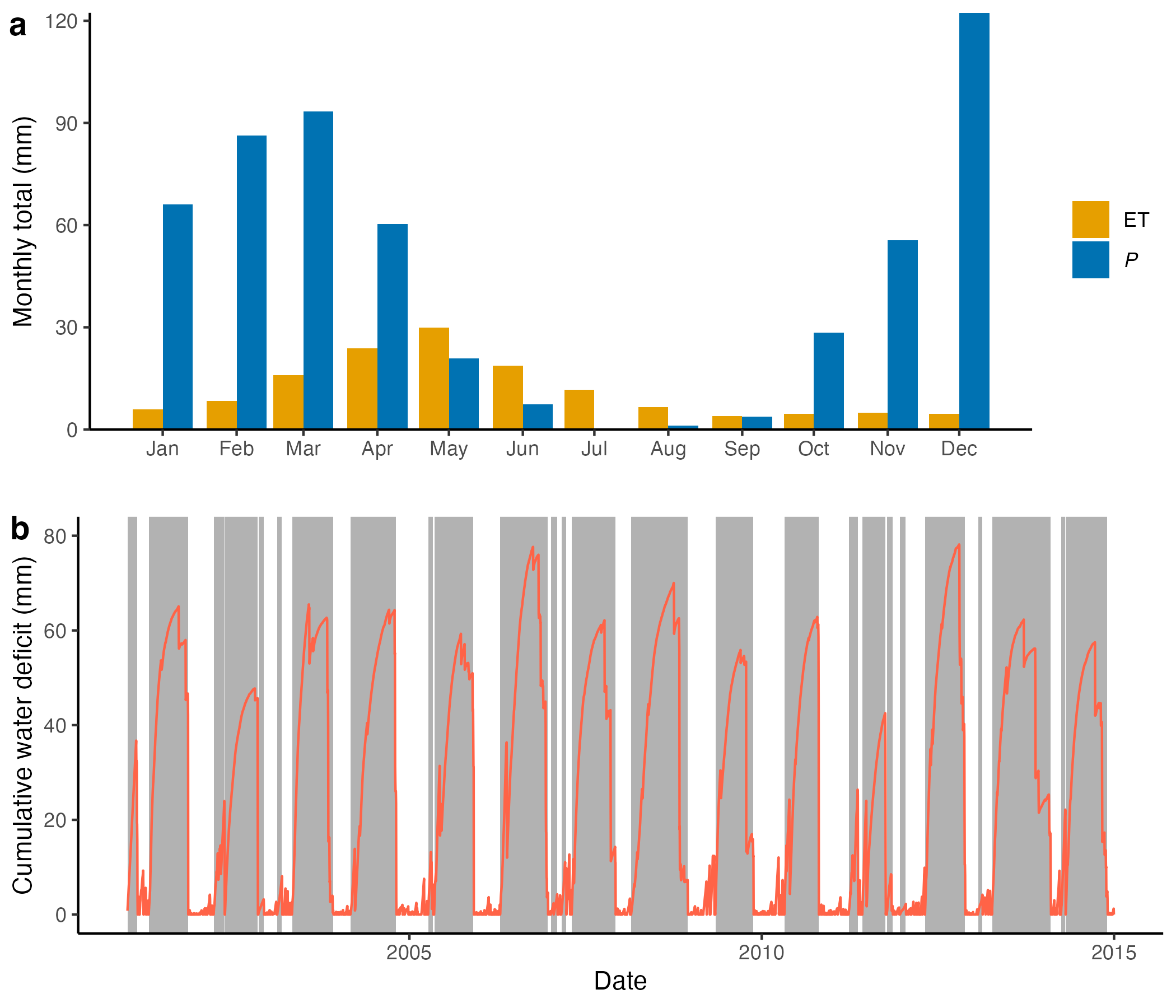
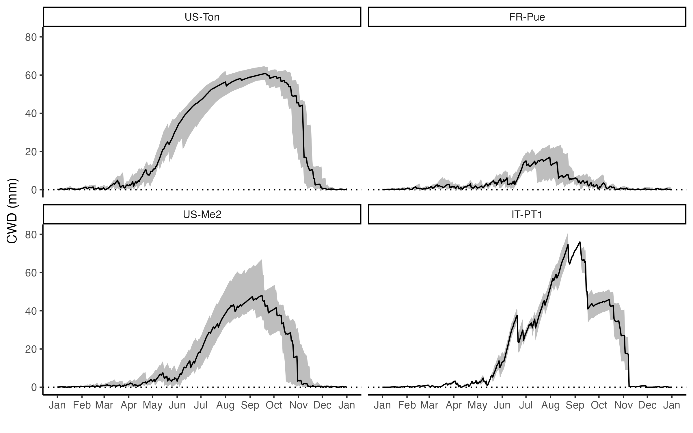
The latent heat flux and precipitation have clear seasonal variations in most biomes. As described above, for annual totals, \(P \geq E\). However, over shorter periods of time, ET may exceed precipitation (\(E > P\)). Of course, on a rain-free day \(P=0\), while \(E>0\). In some climates, \(E > P\) may also be sustained over several weeks to months. For example, in Mediterranean or Monsoonal climates, the asynchroneity of precipitation and solar radiation (and thus net radiation) can create a seasonal imbalance of water and energy availability and thus of water inputs and losses. As an example, Figure 8.4 a shows the multi-year average monthly total precipitation (\(P\)) and ET (the same as \(E\)) for an ecosystem in a Mediterranean climate - a woody savannah in California (eddy covariance measurement site US-Ton). It shows that \(E>P\) on average for May-Sep each year. The difference in monthly totals is relatively small - on the order of 10 mm or less. However, considering the cumulative sum of daily \(E-P\) during the dry summer months for calculating the cumulative water deficit (Figure 8.4 b) shows that the maximum attained seasonal water deficit is 40-80 mm for this site (and varies between years). This is a substantial amount. Where does this water come from? Of course, it’s drawn by plants through their roots from the rooting zone, including the soil and potentially also the sub-soil or even the groundwater. How much water can be stored in the soil is the topic of the next section.
8.3 Soil water
Soils are an important storage component of water. Soil water (or soil moisture) supplies water for plant transpiration and soil evaporation during dry periods. How much soil moisture is accessible to plants determines how rapidly plants experience water stress during dry periods and affects the surface energy partitioning, near-surface air heating and heat extremes. Soil moisture also acts to buffer the asynchroneity of precipitation and radiation (and thus potential evapotranspiration) and introduces an important memory element in the Earth system (Seneviratne et al. 2010). For example, an anomalously dry spring may aggravate water stress later in the season because soil moisture stores that have re-filled during the wet winter (and may still be relatively moist in spring) get depleted gradually and may reach a critically low moisture level earlier than after a wet spring. The strength of this memory effect and the time it takes for plants to experience water stress during dry periods depends (i.a.) on the capacity for plant-accessible water storage in the rooting zone of vegetation.
An important determinant for how much water can be stored in a given volume of soil is its texture. The size of soil particles determines their surface area. Water is adsorbed to the surfaces of the soil matrix and it takes work to remove it. Therefore, the size distribution of soil particles determines how much water the soil can bound. Soil particles are distinguished by size into sand (2-0.05 mm), silt (0.05-0.002 mm), and clay (<0.002 mm). A soil is a mixture of size classes and depending on this mixture, it can be classified into a soil texture class (Figure 8.5).
Code
library(dplyr)
library(ggplot2)
library(ggtern)
library(grid)

# Load the Data. (Available in ggtern 1.0.3.0 next version)
data(USDA)

# Put tile labels at the midpoint of each tile based on https://stackoverflow.com/questions/29136168/add-texture-classes-to-soil-classification-triangle-via-ggplot2
USDA.LAB <- USDA |>
  group_by(Label) |>
  dplyr::summarise(across(where(is.numeric), mean))

# Tweak
USDA.LAB$Angle = 0
USDA.LAB$Angle[which(USDA.LAB$Label == 'Loamy Sand')] = -35

# Construct the plot.
ggplot(data = USDA, aes(y = Clay, x = Sand, z = Silt)) +
  coord_tern(L="x", T="y", R="z") +
  geom_polygon(alpha = 0.75, size = 0.5, color = 'black', aes(color = Label, fill = Label)) +
  geom_text(data = USDA.LAB,
            aes(label = Label, angle = Angle),
            color = 'black',
            size = 3.5) +
  theme_rgbw() +
  theme_showsecondary() +
  theme_showarrows() +
  custom_percent("(%)") +
  theme(legend.position="none") +
  labs(fill  = '',
       color = '')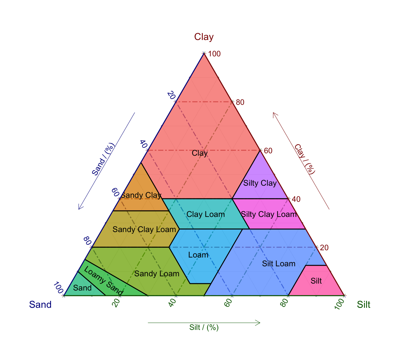
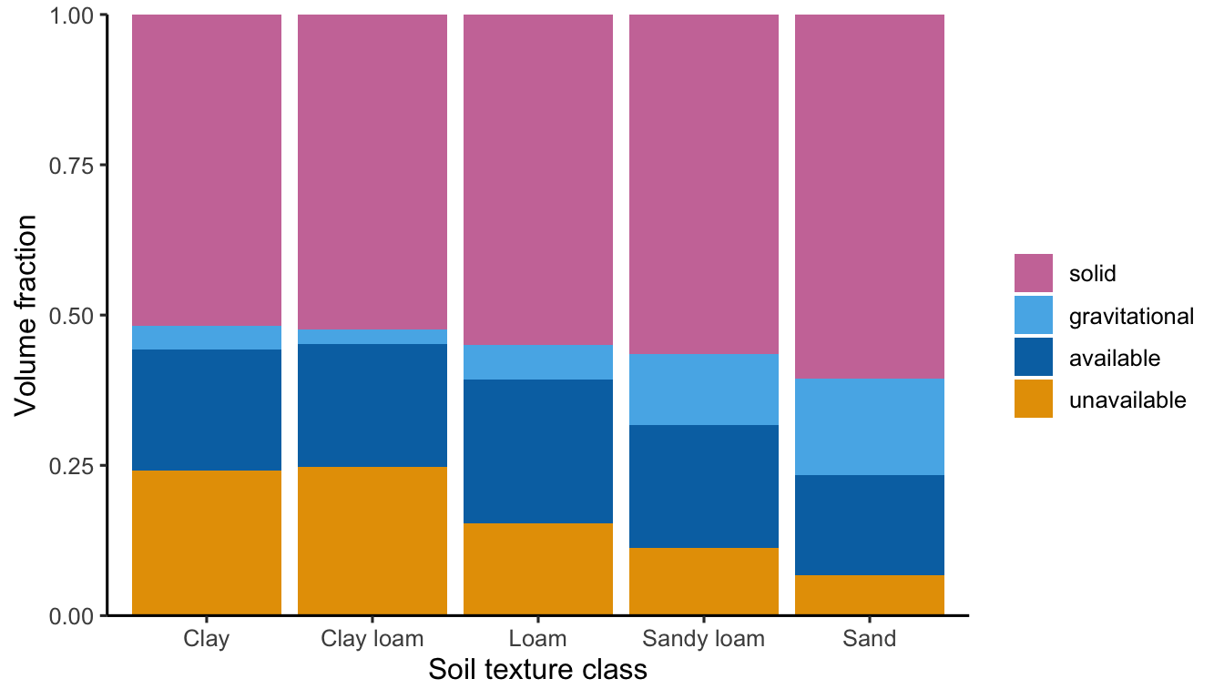
In a common soil (not compacted, not an organic - peatland - soil), about 55% of the volume is comprised of solid material. The rest is air and water. The fraction of the soil that is not solid material is referred to as the porosity. When all pores are filled with water, the soil volumetric water content is at saturation (\(\theta_\text{SAT}\)). Soil texture classes vary relatively little with respect to porosity, but differ strongly in the strength at which the water is adsorbed to the soil matrix (Figure 8.7). Water movement in soil is driven by two distinct forces. The gravitational potential “pushes” water through soil under the influence of gravity. The soil matric potential \(\psi_s\) arises from the adsorption of water to soil particles. It takes work to remove water from their adsorption to the soil matrix.
The matric potential is commonly expressed in units of mm or Pa. It can also be expressed as the suction head which is the negative of the matric potential.
Imagine you stick a straw into the soil and try to suck out the water. When the soil is wet, you initially don’t have to suck hard to withdraw water. The suction head has a small positive value. The matric potential has a small negative value. After you have sucked out some amount water from the soil, you have to start sucking “harder” to extract the same amount again as the soil dries out. That’s because the matric potential declines to more negative numbers (and the suction head increases to larger positive numbers) for drier soils. Staying with the straw analogue, -1 mm matric potential (or 1 mm suction head) is equivalent sucking from your straw such that 1 mm of water doesn’t drain out of the straw (ignoring capillary forces).
The same can also be expressed as a pressure - the gravitational force per unit area: \[ p = \frac{F_G}{A} = \frac{mg}{A} \] 1 mm corresponds to 1 kg m-2 and \(g =\) 9.81 m s-2. Therefore, \[ 1 \; \text{mm} = 9.81 \; \text{kg m}^{-1} \text{s}^{-2} = 9.81 \; \text{Pa} \]
The soil matric potential \(\psi_s\) is related to the soil volumetric water content \(\theta\) in a highly non-linear fashion. It stays near zero for a wide range \(\theta\) and drops off sharply as \(\theta\) falls below a certain range. Reflecting the large variation in how strongly water is bound to the soil matric across different soil texture classes, the relationship \(\psi_s(\theta)\) varies strongly across soil types. An empirical equation for this relationship is given by Clapp and Hornberger (1978) as: \[ \psi_s = \psi_\text{SAT} \left( \frac{\theta}{\theta_\text{SAT}} \right)^{-b} \tag{8.4}\] Here, \(\psi_\text{SAT}\) is the soil matric potential at saturation, that is when \(\theta = \theta_\text{SAT}\). The exponent \(b\) determines how rapidly the matric potential declines towards low \(\theta\). These parameters have different values depending on the soil texture class, resulting in different functional forms of the relationship between volumetric water content and the matric potential.
Code
library(dplyr)
library(readr)
library(ggplot2)
library(cowplot)

# get table of soil parameters by texture class, adopted from Bonan 2015, Table 9.2
df_soilpar <- read_csv(here::here("data/df_soilpar.csv")) |>
  mutate(
    fc_abs = fc * porosity,
    wp_abs = wp * porosity,
    solid = 1 - porosity
  ) |>
  mutate(
    unavailable = wp_abs,
    available = fc_abs - wp_abs,
    gravitational = porosity - fc_abs
  )

calc_psi <- function(swc, soilclass, df_soilpar){
  df_soilpar <- df_soilpar |>
    dplyr::filter(soiltext == soilclass)
  psi <- df_soilpar$psi_sat * (swc / df_soilpar$porosity)^(-df_soilpar$exponent)
  return(psi)
}

drop_by_porosity <- function(swc, psi, soilclass, df_soilpar){
  df_soilpar <- df_soilpar |>
    filter(soiltext == soilclass)
  psi <- ifelse(swc > df_soilpar$porosity, NA, psi)
}

create_df_swc_bysoil <- function(soilclass, df_soilpar){
  tibble(swc = seq(0.01, 1, 0.001)) |>
    mutate(
      soilclass = soilclass
    ) |>
    rowwise() |>
    mutate(
      psi = calc_psi(swc, soilclass, df_soilpar)
    ) |>
    mutate(
      psi = drop_by_porosity(swc, psi, soilclass, df_soilpar)
    )
}

df_swc <- purrr::map_dfr(
  df_soilpar$soiltext,
  ~create_df_swc_bysoil(., df_soilpar)
)

gg1 <- df_swc |>
  ggplot(aes(swc, psi, color = soilclass)) +
  geom_line() +
  geom_hline(yintercept = c(-1000, -150000), linetype = "dotted") +
  khroma::scale_color_okabeito() +
  labs(
    x = "Volumetric soil water content",
    y = expression(paste("Soil matric potential (mm)"))
  ) +
  theme_classic() +
  ylim(-0.5e6, 0) +
  xlim(0, 0.5) +
  theme(legend.position="none")

# # extra plot
# df_swc |>
#   filter(soilclass %in% c("Sand", "Loam", "Clay")) |>
#   ggplot(aes(swc, psi, color = soilclass)) +
#   geom_line() +
#   geom_hline(yintercept = c(-1000, -150000), linetype = "dotted") +
#   khroma::scale_color_okabeito() +
#   labs(
#     x = "Volumetric soil water content",
#     y = expression(paste("Soil matric potential (mm)"))
#   ) +
#   theme_classic() +
#   ylim(-0.5e6, 0) +
#   xlim(0, 0.5) +
#   theme(legend.position="none")
#
# ggsave(here::here("fig/soil_matric_potential_vs_swc.png"), width = 4, height = 3)

gg2 <- df_swc |>
  ggplot(aes(swc, -psi, color = soilclass)) +
  geom_line() +
  geom_hline(yintercept = c(1000, 150000), linetype = "dotted") +
  scale_y_log10() +
  khroma::scale_color_okabeito(name = "Soil texture") +
  labs(
    x = "Volumetric soil water content",
    y = expression(paste("Suction head (mm)"))
  ) +
  theme_classic() +
  xlim(0, 0.5)

plot_grid(
  gg1,
  gg2,
  labels = c("a", "b"),
  rel_widths = c(0.77, 1)
)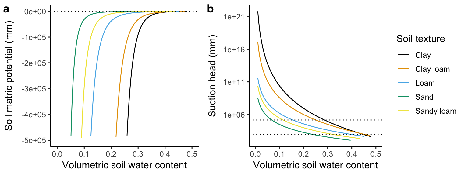
In sandy soils, the size of particles and hence the size of soil pores is large, water is only loosely bound to the soil matrix, and can drain rapidly. The field capacity (\(\theta_\text{FC}\)) is the volumetric water content that is bound to the soil matrix and does not drain due to the gravitational force. Because the matric potential is comparatively low for a given amount of soil water in sandy soils, more water drains due to the gravitational force compared to other soil texture classes. Therefore, \(\theta_\text{FC}\) is lower in sandy soils than in other soils. The higher the field capacity, the more water is retained in the soil and prevented from drainage. However, not all of this water is available for uptake by plants. Depending on the soil texture a certain amount of water is too strongly adsorbed to the soil matrix for plants to “remove” it and mobilise it for uptake through their roots. The permanent wilting point \(\theta_\text{PWP}\) measures the volumetric soil water content that is bound to the soil at a matric potential of -150,000 mm which is taken to be too strongly negative for plants to access. Actually, plants start to respond to water stress by closing their stomates and suffering from damage to their transport vessels already earlier. \(\theta_\text{PWP}\) varies strongly between soil texture classes. It is high for clay soils, meaning that a relatively large amount of soil water remains inaccessible for plant uptake.
Code
library(readr)
library(dplyr)
library(tidyr)
library(ggplot2)

df_soilpar <- read_csv(here::here("data/df_soilpar.csv")) |>
  mutate(
    fc_abs = fc * porosity,
    wp_abs = wp * porosity,
    solid = 1 - porosity
  ) |>
  mutate(
    unavailable = wp_abs,
    available = fc_abs - wp_abs,
    gravitational = porosity - fc_abs
  )

# Volume fractions
df_soilpar |>
  pivot_longer(cols = c(unavailable, available, gravitational, solid)) |>
  mutate(
    name = factor(name, levels = rev(c("unavailable", "available", "gravitational", "solid"))),
    soiltext = factor(soiltext, levels = c("Clay", "Clay loam", "Loam", "Sandy loam", "Sand"))
    ) |>
  ggplot(aes(soiltext, value, fill = name)) +
  geom_bar(position = "stack", stat = "identity") +
  scale_fill_manual(
    name = "",
    values = c(
      "unavailable" = "#E69F00",
      "available" = "#0072B2",
      "gravitational" = "#56B4E9",
      "solid" = "#CC79A7"
    )
  ) +
  scale_y_continuous(expand = c(0, 0)) +
  theme_classic() +
  labs(
    x = "Soil texture class",
    y = "Volume fraction"
)The plant-available soil water holding capacity (WHC) is the difference between the field capacity and permanent wilting point. \[ \text{WHC} = \theta_\text{FC} - \theta_\text{PWP} \] Soil water storage above \(\theta_\text{FC}\) eventually drains and is thus inaccessible for plant uptake and soil water storage water below \(\theta_\text{PWP}\) is too strongly bound to the soil matrix and is therefore inaccessible for plant uptake. WHC is an important measure of suitability of soils for supporting vegetation. A low WHC means that a small amount of water can be stored per soil volume and made available for plant uptake during dry periods. However, the WHC varies only relatively little between soil texture classes as shown in Figure 8.7. This is because \(\theta_\text{PWP}\) and \(\theta_\text{FC}\) are correlated across soil texture classes. Soils with a high \(\theta_\text{FC}\) (clay soils) also tend to have a high \(\theta_\text{PWP}\) and vice versa. However, WHC may vary across different locations also due to other constraints. For example, a large share of gravel (rocks with diameters greater than sand) reduces the WHC.
In view of the relative constancy of WHC, but large variance of \(\theta_\text{PWP}\) and \(\theta_\text{FC}\) across soil texture classes, soil moisture is often expressed as a fraction of available water. The soil water index (also often referred to as the soil water scalar) is commonly defined as \[ W = \frac{\theta - \theta_\text{PWP}}{\theta_\text{FC} - \theta_\text{PWP}} \] Another common expression of soil moisture is in percent saturation (\(100\% \cdot \theta / \theta_\text{SAT}\)).
- Label \(\theta_\text{SAT}\), \(\theta_\text{FC}\), \(\theta_\text{WP}\), porosity, and WHC in Figure 8.7.
8.3.1 Rooting-zone water-storage capacity
All metrics and relationships described above are expressed with a unit soil volume as a reference. For example, the WHC is the amount of water, a given volume of soil can hold. The total amount of water that vegetation has access to - the rooting-zone water-storage capacity \(S_0\) - is determined not only by the soil texture across the rooting zone, but also to rooting depth \(z_r\). It can be conceived as the integral of the WHC across the rooting profile. Assuming a constant WHC across the rooting depth, this is simply \[ S_0 = z_r \cdot \text{WHC}\;. \tag{8.5}\] The rooting depth \(z_r\) is measured in units of length (for example in m), while the WHC is a volume fraction (for example m3 m-3). Hence, \(S_0\) is in units of length. While the WHC varies relatively little across soil texture classes and across different locations globally, rooting depth \(z_r\) varies strongly between species, and plant functional types (Figure 8.8). It tends to be smaller for grasses and forbs than for trees and shrubs.
- Look up species names shown in Figure 8.8 on the internet. Do you know these plants? Do you find patterns that relate to differences between PFTs shown in Figure 8.8 a, and in how the rooting depth relates to the biomes and climate zones in which these species grow?

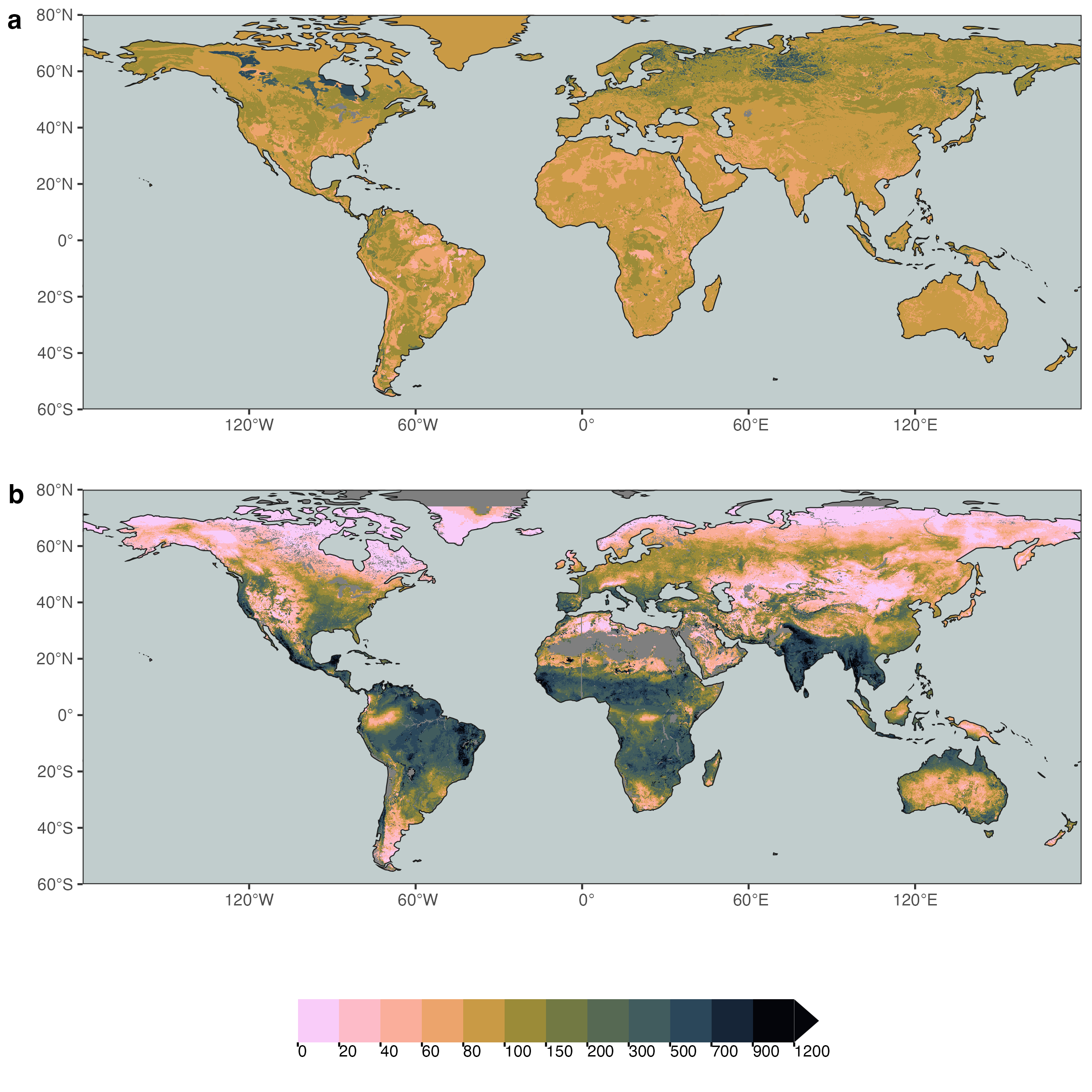
The variations in rooting depth have implications for the rooting-zone water-storage capacity (a consequence of Equation 8.5). This, in turn, variations in \(S_0\) are linked to how sensitive different vegetation types and species respond to dry periods - with consequences for surface energy partitioning is altered as the rooting zone dries out. Variations in rooting depth are related not only to species and PFTs, but also to large-scale climate variations and differences in vegetation cover in the different biomes across the globe (Figure 8.9). As a consequence of the large variations in \(z_r\), the \(S_0\) exhibits a large variation across the globe and its variation is largely disconnected to WHC. In other words, variations in \(S_0\) are primarily driven by \(z_r\), rather than by WHC.
8.4 Plant hydraulics
Water is transported from the soil, across the soil-root interface, and then inside the plant from the fine roots up and along inside the xylem (the water transport vessels) to the leaves. Water evaporates and diffuses through the stomates (Section 4.4). This water transport along the soil-plant-atmosphere (SPA) continuum is a passive process. That is, the plant does not invest energy directly in the process of transporting the water. The water evaporation through leaves is rather an unavoidable “burden” that is traded off against CO2 uptake for photosynthesis (Section 4.4.3).
Have you thought about how water is transported up tall trees? It’s a fascinating aspect of how biology has evolved ways to deal with physics.
The driving force of water transport is the negative pressure that the vapor pressure deficit of the surrounding air creates. This force acts against a resistances and the gravitational force. To move the water up the plant, the water at the level of the leaves is under a strong negative pressure. The taller the plant and the higher the resistance along the soil-plant-atmosphere continuum, the more negative the pressure at the leaf-level to sustain a given water flux (transpiration). This negative water pressure at the level of the leaves is the leaf water potential (\(\psi_l\)). It’s in the same units as the soil matric potential (\(\psi_s\), Equation 8.4) and it is related to the soil water potential via a the transpiration stream \(T\) and an effective whole-plant hydraulic conductance \(G_p\) that considers resistance elements in series - from the soil to the leaf. Remember that a conductance is the inverse of a resistance. In simplified terms, this can be written as. \[ T = -G_p (\psi_l - \psi_s + \rho g h) \tag{8.6}\] \(\rho\) is the density of water (kg m-3), \(g\) is the gravitational constant (9.81 m s-2), and \(h\) is the height of the tree (m), measured from the average depth of the roots to the average height of the leaves. With the units of \(\psi_l\) and \(\psi_s\) in Pa and \(T\) in units of (kg m-2 s-1), \(G_p\) is in units of (s m-1). Equation 8.6 expresses the “supply” of water from the soil. From Equation 4.11, we know how the “demand” for water is determined by the vapor pressure deficit \(D\) and the stomatal conductance \(g_s\). The \(T\) in Equation 8.6 thus has to be equal to the \(T\) from Equation 4.11 (where it was called \(E\)): \[ T = 1.6 \; g_s \; D \tag{8.7}\] These equations illustrate some important points. First, a positive (upward) transpiration stream \(T\) that satisfies the demand from the atmosphere (Equation 8.7) can only be maintained if the leaf water potential is more negative than the soil water potential. Second, as the soil water potential becomes more negative, the leaf water potential also has to become more negative to transport the amount of water that is “demanded” by the atmosphere and determined by \(D\) and \(g_s\). Third, tall trees have to sustain more negative leaf water potentials than short ones for a given soil dryness and transpiration rate. By setting the two equations for \(T\) equal and solving for the leaf water potential \(\psi_l\) also illustrates how soil moisture (\(\psi_s\)) and VPD (\(D\)) have an interactive effect on \(\psi_l\).
Responses of plants to water stress are physiologically triggered through the sensing of leaf water potentials. In other words, \(\psi_l\) is the central quantity that drives water stress responses of plants. Understanding how \(\psi_l\) responds to environmental factors is thus key to understanding how water stress (stomatal closure, damaging drought stress) is a function of soil and air dryness, modified by plant hydraulic traits determining \(G_p\).
Equation 8.6 is a simplification because the whole-plant hydraulic conductance \(G_p\) is a non-linear function of the water potential which drops along the transport pathway from \(\psi_s\) to \(\psi_l\). As a consequence, the interactive effect of VPD and soil moisture is non-linear. To account for the conductance drop with negative water potential, a more realistic form of Equation 8.6 can be written as \[ T = -G_{p,0} \int_{\psi_s}^{\psi_l - \rho g h} P(\psi) \; \text{d}\psi \;, \tag{8.8}\] where \(G_{p,0}\) is a “base” conductance at zero water potential and \(P(\psi)\) is a vulnerability function of the plant conductance. The latter declines towards more negative water potentials. A commonly used functional form is \[ P(\psi) = 0.5^{(\psi/P_{50})^b} \;, \tag{8.9}\] where \(P_\text{50}\) is the water potential at which \(P\) has dropped to 0.5.
Code
library(ggplot2)

vulnerability_curve <- function(psi, p50, b){
  0.5 ^ ((psi/p50)^b)
}

ggplot() +
  geom_function(fun = function(x) vulnerability_curve(x, -2000, 3)) +
  xlim(-4000, 0) +
  geom_vline(xintercept = c(-2000, 0), linetype = "dotted") +
  labs(x = expression(paste(psi, " (Pa)")),
       y = expression(paste(italic(P(psi))))) +
  theme_classic()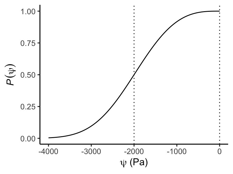
Equation 8.8 can be regarded as the hydraulic supply function for transpiration (Sperry and Love 2015) and Equation 8.9 is commonly referred to as the hydraulic vulnerability curve (Tyree and Sperry 1989). The non-linearity arising from the latter implies that transpiration initially increases with an increasingly negative leaf water potential, but reaches a maximum beyond which transpiration does not further increase despite increasingly negative leaf water potentials. Reaching this point is risky for plants as it bears the danger of potentially lethal hydraulic failure (see below). Stomatal regulation acts to limit leaf water potentials reaching this point, while maximally exploiting soil water that is available for plant uptake without a substantial flattening of the \(T(\psi_l)\) curve. What exactly “substantial” means, depends on plant strategies that vary between species.
Code
library(dplyr)

hydraulic_supply <- function(psi_leaf, psi_soil, g_plant, p50, b){
  transpiration <- -g_plant *
    integrate(
      f = vulnerability_curve,
      lower = psi_soil,
      upper = psi_leaf,
      p50 = p50,      # argument for f
      b = b           # argument for f
      )$value
  return(transpiration)
}

tmp <- expand.grid(
  psi_leaf = seq(-4000, 0, by = 50),
  psi_soil = seq(-2000, 0, by = 100)
) |>
  as_tibble() |>
  rowwise() |>
  mutate(
    transp = hydraulic_supply(
      psi_leaf = psi_leaf,
      psi_soil = psi_soil,
      g_plant = 1e-6,
      p50 = -2000,
      b = 3
      )
  )

tmp |>
  ggplot(aes(x = -psi_leaf, y = transp, color = psi_soil, group = psi_soil)) +
  geom_line() +
  scale_color_viridis_c(
    name = expression(paste(psi[soil], " (Pa)")),
    option = "cividis",
    direction = -1
  ) +
  labs(x = expression(paste(-psi[leaf], " (Pa)")),
       y = expression(paste(italic(T), " (mm s"^-1, ")"))) +
  ylim(0, NA) +
  theme_classic()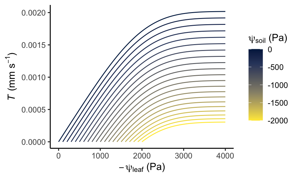
Sustaining very negative water potentials along the transport pathway can be dangerous for the plant. As described in the box above, the whole-plant conductance declines with increasingly negative water potentials. This is because the very negative water potentials can only be sustained if no air is in contact with the water inside the xylem. As pressures become very negative, air may seep in and create embolisms. If the conductance was to drop towards zero, transpiration would collapse and embolisms would be excessive - creating potentially irreversible damage and triggering branch and eventually tree mortality due to hydraulic failure.
Plants can avoid such water stress and hydraulic failure through stomatal regulation (see also Section 4.4.3). To avoid embolisms, stomata close (stomatal conductance is reduced) when the soil water potential declines to increasingly negative values. As a consequence, transpiration, as well as CO2 assimilation, decline. Once soil moisture across the rooting zone is depleted and the soil water potential reach very negative values, vegetation activity (transpiration and assimilation) comes to a halt. However, this rarely happens since water loss cannot be fully avoided even if stomata are fully closed and plants have evolved adaptations and are adjusted through plasticity in various traits to avoid a complete depletion of moisture stores across the rooting zone and to limit water losses. Variations in rooting depth are an expression of this adaptation and acclimation. Leaf properties with thick, waxy leaves that prevent water loss, or a drought-deciduous strategy are other examples.
Different plant species respond differently to water stress (variations in soil water potential) and are characterised with different hydraulic traits that determine the stomatal response to soil and leaf water potentials. Two examples are shown in Figure 8.12
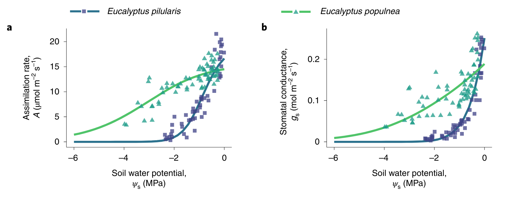
- Consider a soil dry down as in Figure 8.12. Sketch qualitatively how the following variables change as a function of the soil water potential (while all other meteorological variables remain constant):
- Soil water content
- Latent heat flux
- Sensible heat flux
- Bowen ratio
- Evaporative fraction
- GPP
- Reco
- NEE
- Tree mortality due to hydraulic failure
8.5 Water bucket model and ecohydrological relations
In this and in the previous chapter (Chapter 7), we have learned about three important points that follow from mass and energy conservation and govern the water balance and its components:
- Precipitation \(P\) is partitioned into evaporation \(E\) and runoff \(R\), as described by the ecosystem water balance (Equation 8.2).
- Evaporation is limited by the amount of available water in the rooting zone (Section 8.3 and Section 8.4). As the soil across the root-penetrated depth dries out, \(E\) declines towards zero. If there is no water available, there can be no transpiration or evaporation.
- Evaporation is also limited by the amount of energy that is available at the land surface for evaporating water. This is described by the dependence of the potential evapotranspiration on net radiation (Section 7.2.1).
A fourth point is:
- Once the soil is water-saturated, it has no more capacity for absorbing \(P\) and storing the water, and \(P\) is diverted to runoff (\(R\)).
A simple model that considers these four points is to conceive the ecosystem water balance with the bucket model, whereby the rooting zone water storage capacity is determined by a “bucket depth”, given by \(S_0\) (Equation 8.5). Precipitation fills the bucket up to its maximum capacity \(S_0\). Once the bucket is full, additional precipitation goes into runoff, while runoff is zero before the bucket is full. The water-unlimited rate of \(E\) is PET. \(E\) is drawn from the water stored in the bucket and the actual ET (here \(E\)) is reduced as a function of the remaining water in the bucket: \[ E(t) = \text{PET}(t) \frac{S(t)}{S_0} \tag{8.10}\] Runoff is generated only when the bucket is full. \[ R(t) = \begin{cases} P(t) - (S_0 - S(t)) \; & \forall \; P(t) \geq S_0 - S(t) \\ 0 \; & \forall \; P(t) < S_0 - S(t) \end{cases} \] The soil water balance, i.e., the change in the root zone water storage \(S\) is given by the balance of water inputs (\(P(t)\)), and losses (ET: \(E(t)\) and runoff: \(R(t)\)): \[ \frac{\text{d}S}{\text{d}t} = P(t) - E(t) - R(t) \tag{8.11}\] Note that \(S(t)\) is the total soil water content across the rooting zone. It is related to \(\theta\) as \(S(t) = z_r \theta(t)\).
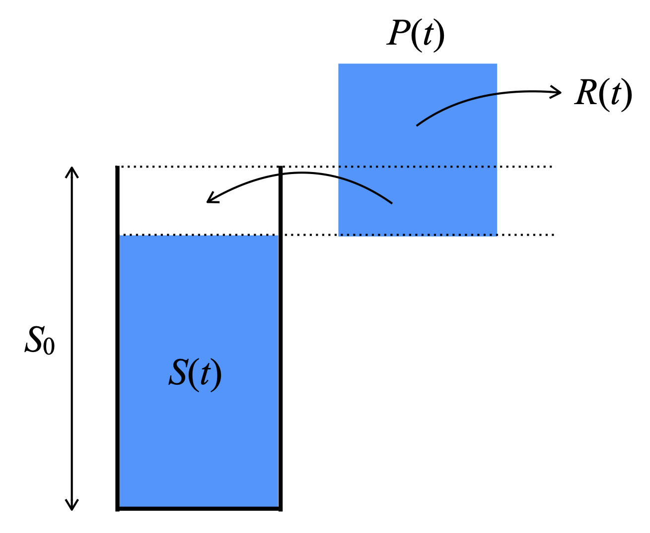
From these four points, several key ecohydrological relations, governing the relation of ecosystem water and energy fluxes over time and across the globe, follow.
Energy and water-limited ecosystems
In wet climates, where the soils are perennially moist (\(S(t)/S_0\) mostly around 1), ET is driven by net radiation (as expressed through PET(Rn), Equation 7.6). Such ecosystems are therefore referred to as energy-limited and the annual total acutal ET (AET) is close to the annual total PET.
In water-limited ecosystems, the annual total ET is substantially lower than the annual total PET. However, not just annual totals of net radiation and precipitation matter, but also their distribution over days and over the seasons (see below).
Figure 8.14 shows AET for different combinations of precipitation and PET. Given sufficient precipitation, AET is close to PET and curves are close to the 1:1 line. Ecosystems located in this part of the domain are referred to energy-limited. If P falls below PET, AET drops below PET. Such ecosystems are water-limited. The ratio of P/PET is (sometimes) referred to as the moisture index. Its inverse, PET/P is often referred to as the aridity index (But beware: sometimes the two former is called ‘aridity index’ in the literature). A site’s or an ecosystem’s aridity is commonly quantified by P/PET, considering annual totals as done in Figure 8.14.
Code
library(ggplot2)

# data created in analysis/analyse_waterbucketmodel.R
df_pet <- readRDS(here::here("data/df_pet.rds"))

df_pet |>
  ggplot(
    aes(
      x = pet,
      y = aet,
      group = prec,
      color = prec
    )
  ) +
  geom_line() +
  geom_abline(slope = 1, intercept = 0, linetype = "dotted") +
  theme_classic() +
  scale_color_viridis_c(
    name = expression(paste(italic("P"), " (mm)")),
    option = "magma"
  ) +
  coord_equal() +
  labs(
    x = "PET (mm)",
    y = "AET (mm)"
  )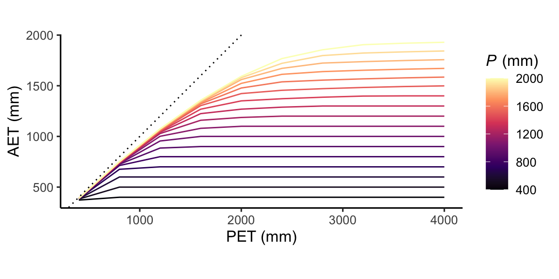
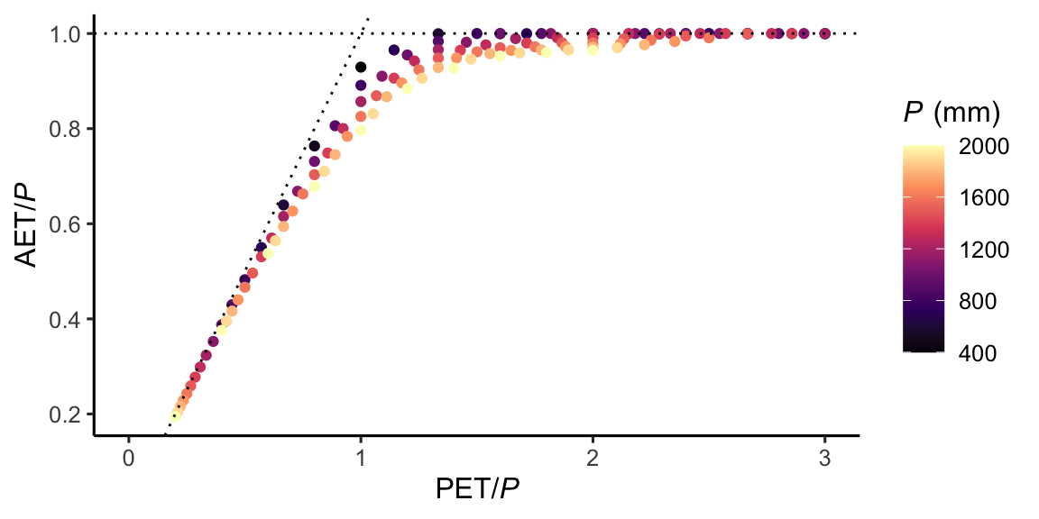
Figure 8.14 illustrates that for high PET in relation to P, AET is close to P. In other words, given sufficient energy, all available water that falls as precipitation is consumed by AET. By dividing the x-axis and the y-axis of Figure 8.14 by P, we control for the effect of P on AET. The resulting relationship has a useful interpretation. It means that we can estimate the fraction of P that gets “consumed” by AET as a function of the aridity index.
The emerging pattern is known as the Budyko relationship. It illustrates how, for energy-limited systems towards the left end of the x-axis, AET increases with energy availability (measured by PET), largely independent of P. Towards the right end of the x-axis are the water-limited systems. Here, PET is much larger than P and all available water gets consumed by AET. In between, there is a range of AET/P values for a given aridity index. The higher the precipitation (in relation to the root zone water storage capacity), the lower AET/P. This is because a larger share is diverted to runoff if precipitation is high and cannot be stored in the limited storage capacity along the rooting zone.
Code
# Budyko
df_pet |>
  ggplot(
    aes(
      x = pet/prec,
      y = aet/prec,
      color = prec
    )
  ) +
  geom_point() +
  geom_abline(slope = 1, intercept = 0, linetype = "dotted") +
  geom_hline(yintercept = 1, linetype = "dotted") +
  scale_color_viridis_c(
    name = expression(paste(italic("P"), " (mm)")),
    option = "magma"
  ) +
  theme_classic() +
  xlim(0, 3) +
  labs(
    x = expression(paste("PET/", italic(P))),
    y = expression(paste("AET/", italic(P)))
  )
ET decay
During rain-free periods, E(t) gradually declines from its initial value. The shape of this decline over time roughly has the shape of an exponential decay (Teuling et al. 2006). The decay rate is determined by PET (thus Rn) and the rooting-zone water-storage capacity S0.
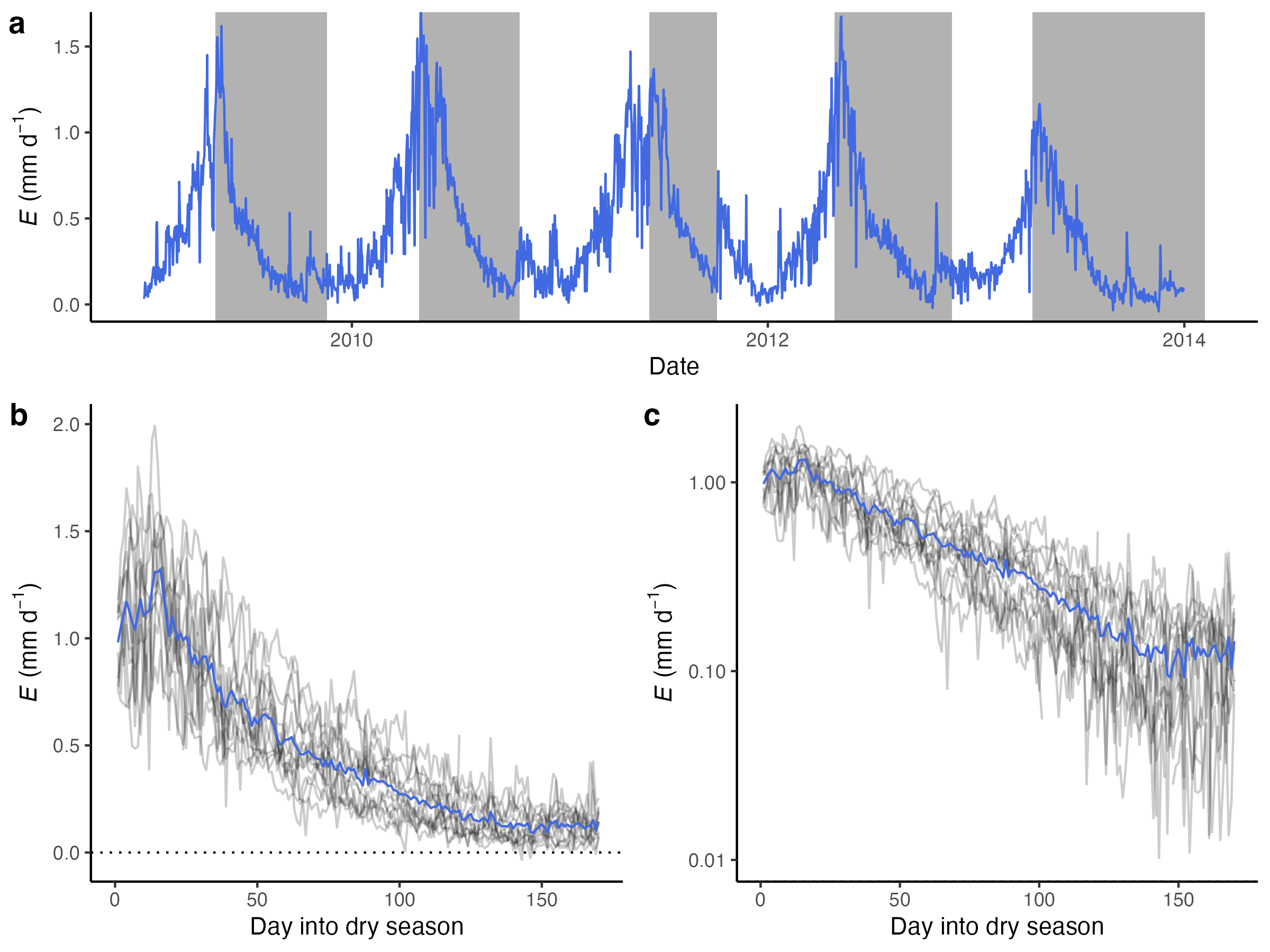
The exponential shape of the ET decline during dry periods directly follows from the water bucket model as defined above. During dry (rain-free) periods, \(P=0\) and no runoff is generated (\(R=0\)). Equation 8.11 simplifies to \[ \frac{\text{d}S}{\text{d}t} = - E(t) \] With Equation 8.10: \[ \frac{\text{d}S}{\text{d}t} = - \frac{\text{PET}(t)}{S_0} \; S(t) \] Assuming that PET is constant, this equation describes a simple first-order decay and is solved by and the following exponential function: \[ S(t) = S_\text{init} \exp \left(-\frac{\text{PET}}{S_0} \; t \right) \] Here, the rate constant of the exponential decay is \(\text{PET}/S_0\). In other words, the higher PET, the more rapid the decline. The higher S0, the slower the decay.
Rooting-zone water-storage as a buffer
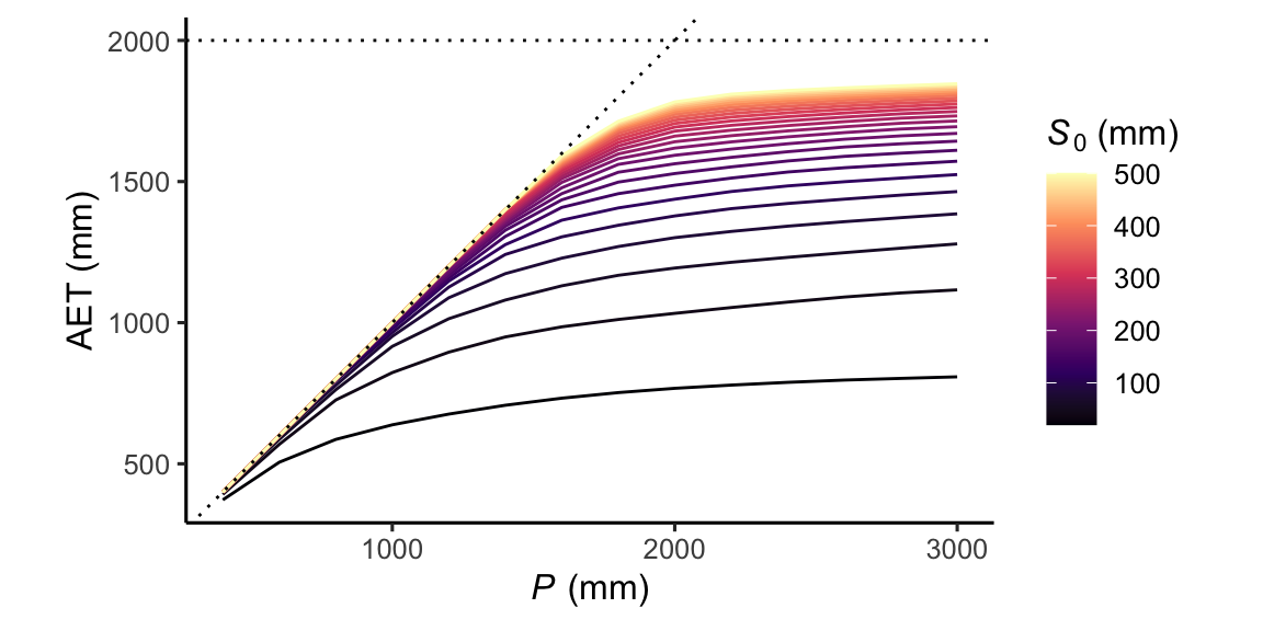
The rooting-zone water-storage capacity S0 “buffers” variations in precipitation and determines how much moisture is plant-available during rain-free periods. Rooting depth, through its influence on S0, thus has the effect of compensating asynchroneities between water supply through precipitation and demand via PET (thus Rn). A larger S0 implies a higher ratio of annual total ET over annual total P.
Code
library(ggplot2)

# data created in analysis/analyse_waterbucketmodel.R
df_s0 <- readRDS(here::here("data/df_s0.rds"))

df_s0 |>
  ggplot(
    aes(
      x = prec,
      y = aet,
      group = s0,
      color = s0
    )
  ) +
  geom_line() +
  geom_abline(slope = 1, intercept = 0, linetype = "dotted") +
  geom_hline(yintercept = 2000, linetype = "dotted") +
  theme_classic() +
  scale_color_viridis_c(
    name = expression(paste(italic("S")[0], " (mm)")),
    option = "magma"
  ) +
  coord_equal() +
  labs(
    x = expression(paste(italic(P), " (mm)")),
    y = "AET (mm)"
  )
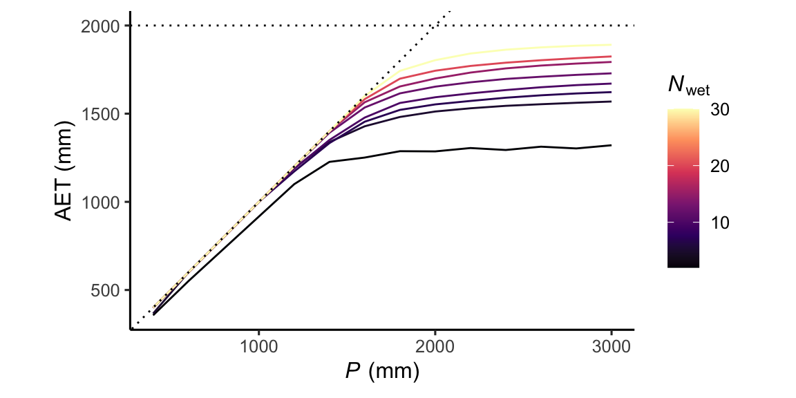
Rainfall distribution
The distribution of rain over time matters. A “constant drizzle” keeps the bucket moist throughout the year and ET will stay close to PET. In contrast, if all annual precipitation falls within a short period of time, the bucket is quickly saturated and a higher fraction of the annual precipitation goes into runoff. In that case, some time after the large rainfall event or the short but intense moist season, the soil dries out again because the excess water has not been stored, and ET starts falling below PET.
If part of the precipitation falls as snow, the timing of its melting and infiltration as liquid water into the rooting zone matters. Snow melt water can be a substantial root zone moisture input during months when \(P-E\) is already negative (for example late spring in the Sierras of California).
Code
library(ggplot2)

# data created in analysis/analyse_waterbucketmodel.R
df_wetd <- readRDS(here::here("data/df_wetd.rds"))

df_wetd |>
  filter(mwetd != 3) |>
  ggplot(
    aes(
      x = prec,
      y = aet,
      group = mwetd,
      color = mwetd
    )
  ) +
  geom_line() +
  geom_abline(slope = 1, intercept = 0, linetype = "dotted") +
  geom_hline(yintercept = 2000, linetype = "dotted") +
  theme_classic() +
  scale_color_viridis_c(
    name = expression(paste(italic(N)[wet])),
    option = "magma"
  ) +
  coord_equal() +
  labs(
    x = expression(paste(italic(P), " (mm)")),
    y = "AET (mm)"
  )
Seasonality of radiation and precipitation
The seasonality of Rn and P matters. If P is high in months when Rn is high, soils remain moist, and ET stays close to PET. In contrast, when Rn is high during the dry period of the year, and Rn is low during the moist period of the year (e.g., in Mediterranean climates), a relatively large fraction of annual total P goes into runoff despite the ecosystem being water-limited during the dry period of the year. This is the case in Mediterranean climates where the dry period can extend over several months (Figure 8.4).
The model described here is a simplification. What empirically known aspects of the ecosystem water balance are ignored in terms of …
- runoff generation
- the dependence of \(E\) on \(S(t)\)
…?
8.6 Ecosystem water fluxes
Water limitation has effects on stomatal conductance through plant hydraulic relations (Section 8.4) and on the amount of active green leaves, measured by the LAI or - from space - by surface greenness indices (Section 6.2). This affects the surface conductance to water vapor and, in turn, the surface energy partitioning (Section 7.2.2). To illustrate the effects of water limitation on the partitioning of net radiation into the turbulent heat fluxes \(H\) and \(\lambda E\), let’s compare the measured fluxes at four temperate sites (Figure 8.19) with a warm and relatively dry summers.
Code
df_sites <- read_csv(here::here("data/fdk_site_info.csv"))

# chose representative sites
use_sites <- c(
      "US-Ton", # Woody savannah, strong sensitivity
      "FR-Pue", # Evergreen broadleaved, strong sensitivity
      "US-Me2", # Evergreen needleleaved, low sensitivity
      "IT-PT1"  # Deciduous broadleaved, low sensitivity
    )

# subset data
df_sites |>
  filter(sitename %in% use_sites) |>
  mutate(
    lon = format(lon, digits = 3),
    lat = format(lat, digits = 3),
    elv = format(elv, digits = 3)
    ) |>
  select(
    Site = sitename,
    Longitude = lon,
    Latitude = lat,
    Elevation = elv,
    `Vegetation type` = igbp_land_use,
    `Climate zone` = koeppen_code
    ) |>
knitr::kable()| Site | Longitude | Latitude | Elevation | Vegetation type | Climate zone |
|---|---|---|---|---|---|
| FR-Pue | 3.60 | 43.7 | 270 | EBF | Csa |
| IT-PT1 | 9.06 | 45.2 | 60 | DBF | Cfa |
| US-Me2 | -121.56 | 44.5 | 1253 | ENF | Csb |
| US-Ton | -120.97 | 38.4 | 177 | WSA | Csa |
All four sites experience cumulative water deficits during the summer months (Figure 8.20) - albeit to a varying degree.
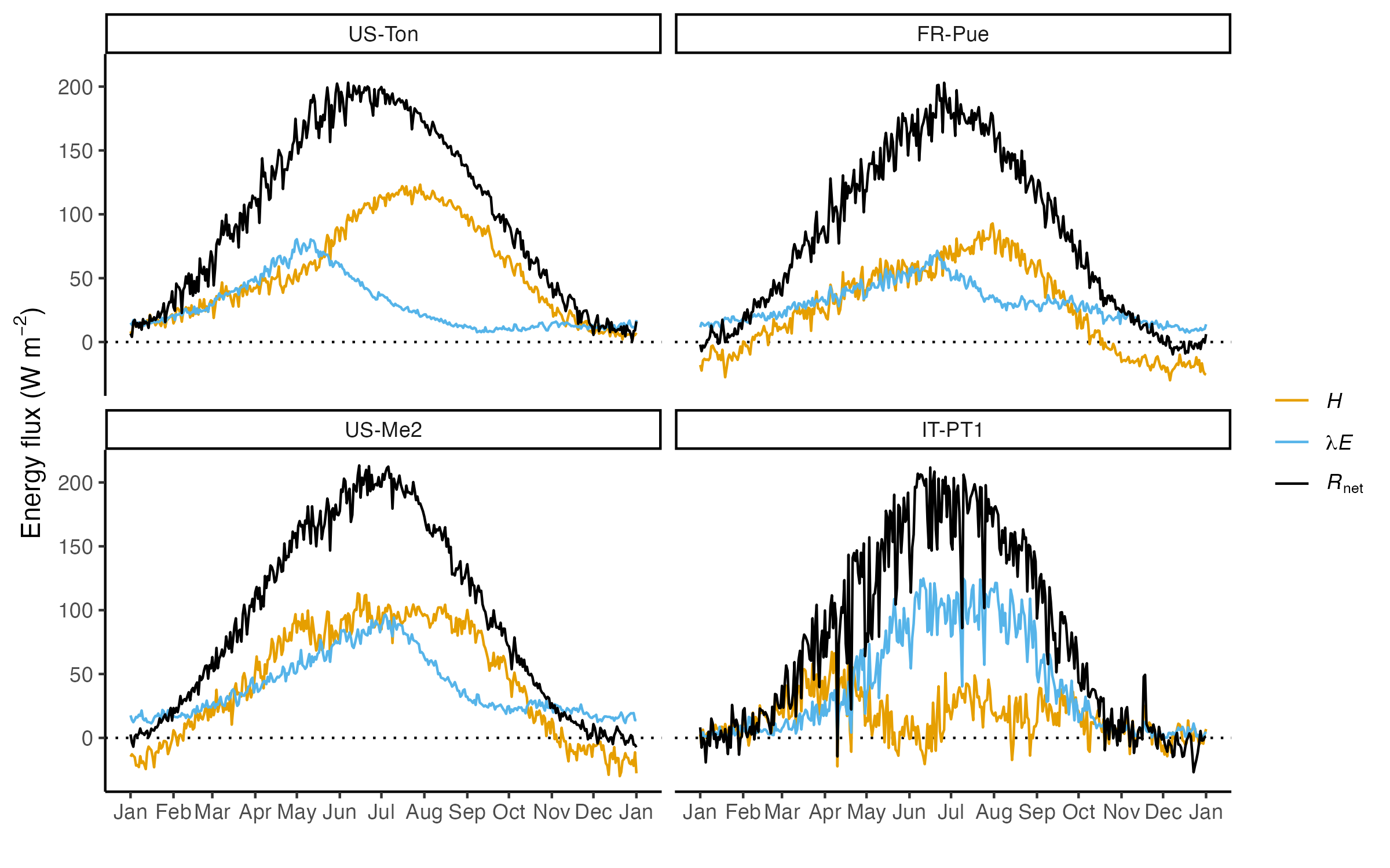
- How does the Bowen ratio and the evaporative fraction change throughout the year at the four sites? Do you see a characteristic pattern of these four sites with relatively dry summers compared to the three temperate sites with relatively moist summers shown in Figure 7.12?
- Compare US-Ton and IT-PT1. At both sites, net radiation reaches around 200 W m-2, yet the seasonal course of \(H\) differs. Why?
- Compare US-Ton and IT-PT1. The seasonal course of \(\lambda E\) differs between the two sites. What could be a reason?
- The energy partitioning, measured by the Bowen ratio, is similar at US-Me2 and FR-Pue, yet the two sites differ with respect to their average cumulative water deficits. What could be a reason?
8.7 Energy and water limitation across the globe
Ecosystems are commonly distinguished into energy-limited and water-limited systems. This notion relates to the dominant limiting resource and to the relations described in Section 8.5. When the bucket is full, the system is energy-limited. When it gets depleted, the system becomes water-limited. Of course, this is a simplification. The relations described in Section 8.5 really refer to a spectrum, rather than a binary classification.
Furthermore, water-limited conditions may be temporally limited and interspersed by energy-limited periods. Also, the water bucket model, as formulated above, suggests that water-limitation sets in at the point when soil moisture falls below the field capacity. However, as long as the net radiation and the atmospheric vapor pressure deficit are not “excessive”, the demand for transpiration (Equation 8.7) may be met by the supply (Equation 8.8) without substantial stomatal closure during the daytime.
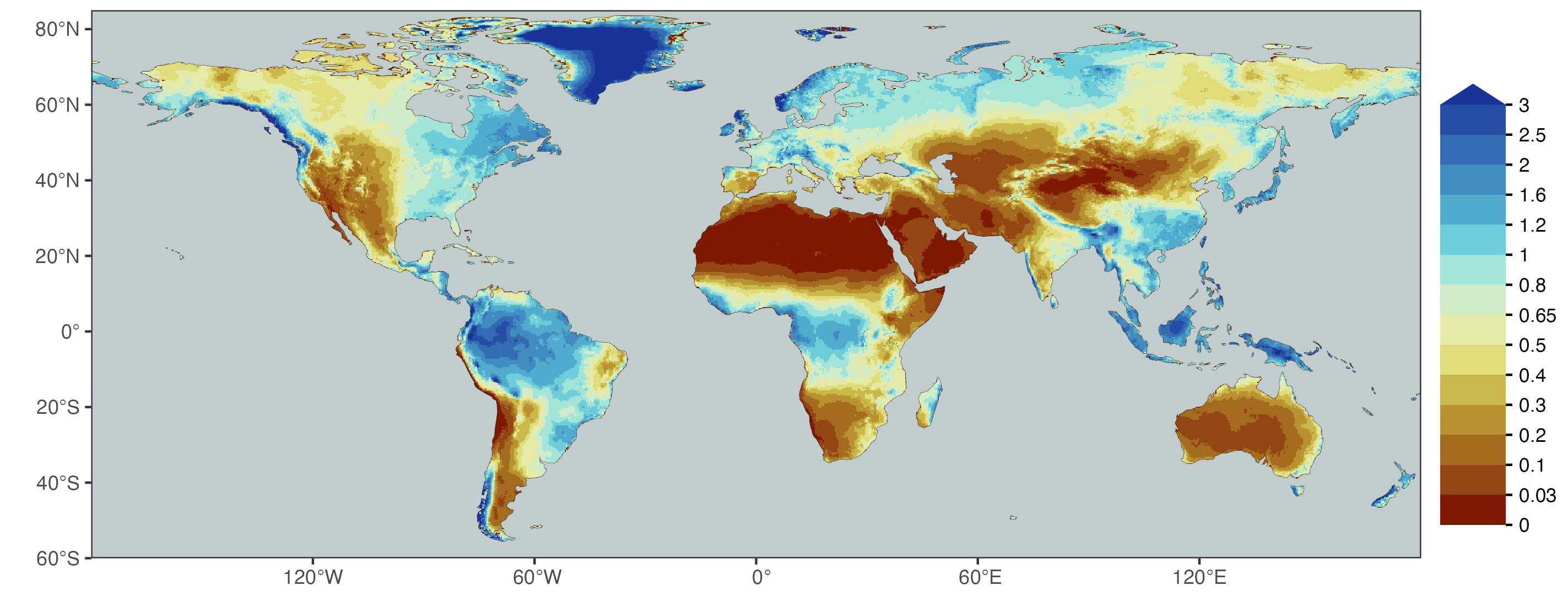
A common classification of ecosystems into aridity classes is given in Table 8.1 based on Middleton and Thomas (1992). This considers the moisture index as defined by P/PET.
| Moisture index value | Aridity class |
|---|---|
| <0.03 | Hyper arid |
| 0.03-0.2 | Arid |
| 0.2-0.5 | Semi-arid |
| 0.5-0.65 | Dry sub-humid |
| >0.65 | Humid |
The global distribution of the moisture index (Figure 8.22) resembles global distributions of vegetation patterns (Section 2.5). In regions where radiation (and temperature) does not limit vegetation, it may additionally be limited by water, as reflected by the moisture index and its low values across the worlds drylands.
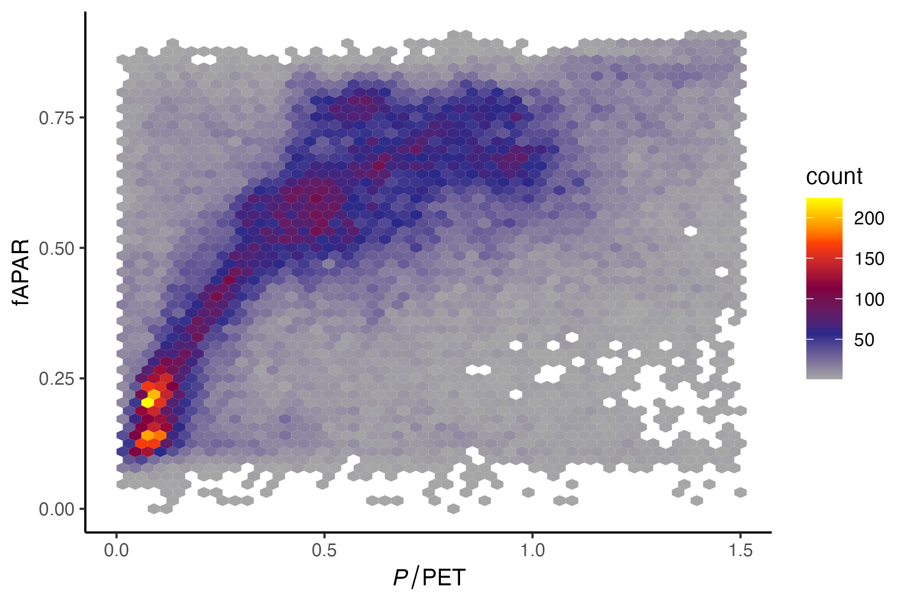
When combining the data for the satellite remote-sensing based fAPAR and the moisture index, a similar pattern emerges as described in Section 8.5. The green vegetation cover, measured by fAPAR, initially increases linearly with increasing P/PET for low values of the latter. Beyond a certain value, fAPAR no longer shows a relationship with P/PET (Figure 8.23).
The slope of the initial linear increase of fAPAR vs. P/PET reflects the water-carbon coupling. The amount of active green and transpiring foliage area is limited by water availability. research has shown that the relationship shown in Figure 8.23 is shifting such that the slope of the initial increase tends to steepen over time (Donohue et al. 2013; Ukkola et al. 2016). This is related to the fact that under rising CO2, stomatal conductance tends to increase (Figure 4.11) and the water use efficiency is enhanced (Section 4.4.1). In other words, a larger area of green leaves per unit ground area can be sustained for a given level of aridity.
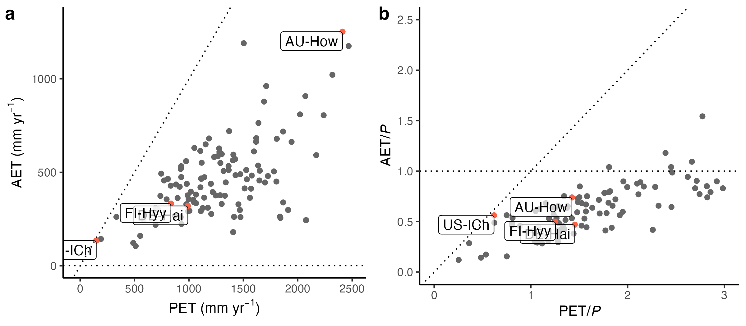
Related patterns emerge from the annual sums of ecosystem water fluxes (AET, PET, and P) measured from surface-atmosphere exchange (eddy covariance technique, Figure 8.24). However, at the scale at which ecosystem fluxes are measured (~1 km2), AET is sometimes larger than precipitation, as suggested by Figure 8.24 (b). This may be related to errors in precipitation and latent heat flux estimates, or due to vegetation having access to the groundwater and/or being supplied moisture through lateral subsurface flow.
8.8 Landscape-scale heterogeneity
Coming soon.
