4 Phenology trends
4.1 Introduction
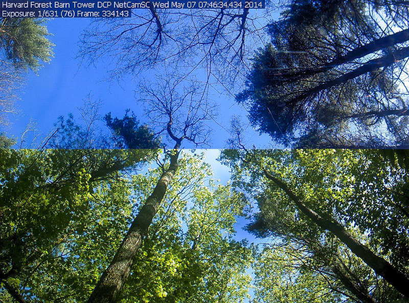
Phenology is broadly defined as seasonally recurring life cycle events, ranging from migration to seasonal plant growth. Land surface phenology is a first order control on the exchange of water and energy between the biosphere and atmosphere (Cleland et al. 2007; Lieth 2013; Piao et al. 2019; Richardson et al. 2010). With phenology being sensitive to temperature, it can be considered an indicator of climate change (Peñuelas and Filella 2009). Plant phenology has historically been recorded for many centuries (Menzel and Dose 2005). More recently, plant phenology (and its changes) have been recorded by networks of observers (Crimmins et al. 2017), near-surface cameras (Richardson 2018; Richardson et al. 2018), and by global satellite monitoring (Zhang et al. 2003; Ganguly et al. 2010).
All these (remote sensing) measurements have provided us with insights in how climate change has altered plant phenology. Overall, climate change drives temperatures up, and moves the phenology of leaf-unfolding by deciduous trees in winter-cold climates (temperate and boreal forest ecosystems) forward in time (from spring toward winter) at a rate of ~ 1 - 5 days per decade, with rates varying depending on locality and altitude (Wang et al. 2015; Vitasse et al. 2009; Menzel et al. 2006).
Consequences are manyfold, such as exposing early blooming or leafing plants to an increased risk of late frost events and related damage to leaves (Hufkens, M. A. Friedl, et al. 2012; Augspurger 2013; Gu et al. 2008). In short, changes to plant and land surface phenology have a profound effect on both the carbon balance and all (co-) dependent processes (Hufkens, M. A. Friedl, et al. 2012). Therefore, it is key that we can detect and quantify how phenology changes in response to year-to-year variability in temperatures, and long-term trends related to anthropogenic climate change and global heating (Richardson et al. 2010; Peñuelas and Filella 2009).
Satellite remote sensing data products provide these insights for almost four decades (Zhang et al. 2003; Hufkens, M. Friedl, et al. 2012). Remote sensing products of land surface phenology provide wall-to-wall coverage with a relatively high level of data consistency across space and time and well-studied known (methodological) biases. This chapter covers several aspects of developing a small research project using remote sensing data of surface phenology, gathered for a small set of locations (a handfull of pixels).
This chapter (Chapter 4) highlights how to detect landscape-wide trends in phenology and how they relate to topography (elevation, aspect) and land cover type. This knowledge can then be used to infer some general properties of vegetation phenology. Chapter Chapter 5 demonstrates how you can detect phenological dates (timing of leaf-unfolding) from vegetation time series yourself, using a simple algorithm, and scale this regionally and globally. Note that throughout the phenology chapters I use phenology and leaf-out interchangeably (depending on the context).
Now, let’s get started!
4.2 Getting the required data
To detect and quantify relationships between phenology and topography, we require relevant data sources. Various sources can be found online but the easiest is to use the geodata package which provides a way to access Shuttle Radar Topography Mission (SRTM) elevation data (digital elevation model, DEM) easily. The below command downloads DEM tiled data from the larger Bern area, as specified by a latitude and longitude.
# load libraries
library(geodata)

# download SRTM data
# This stores file srtm_38_03.tif in
# subfolder elevation of tempdir()
geodata::elevation_3s(
    lat = 46.6756,
    lon = 7.85480,
    path = tempdir()
  )

# read the downloaded data
# use file.path() to combine
# a directory path with a filename
dem <- terra::rast(
  file.path(
    tempdir(),
    "elevation",
    "srtm_38_03.tif"
    )
)
In this exercise, we will rely on the MODIS land surface phenology product (MCD12Q2). This remote sensing-based data product quantifies land surface phenology and is a good trade-off between data coverage (global) and precision (on a landscape scale).
To access this data, we will use the MODISTools package. See Chapter Chapter 2 for an in depth discussion on accessing data using APIs and the MODISTools API in particular. Data is downloaded here for the same location as used for the elevation data above.
# load libraries
library(MODISTools)

# download and save phenology data
phenology <- MODISTools::mt_subset(
  product = "MCD12Q2",
  lat = 46.6756,
  lon = 7.85480,
  band = "Greenup.Num_Modes_01",
  start = "2012-01-01",
  end = "2012-12-31",
  km_lr = 100,
  km_ab = 100,
  site_name = "swiss",
  internal = TRUE,
  progress = FALSE
)
NoteNote
It is always important to understand the data products you use. Find information on who produced the product, track down the latest literature in this respect and note what the limitations of the product are.
- What does the band name stand for?
- How does this relate to other bands within this product?
- What are the characteristics of the downloaded data?
- is post-processing required?
Write down all these aspects into any report (or code) you create to ensure reproducibility.
The downloaded phenology data and the topography data need post-processing in our analysis. There are a number of reasons for this:
- MODIS data comes as a tidy data frame
- MODIS data might have missing values
- DEM data extent is larger than MODIS coverage
- Two non-matching grids (DEM ~ MODIS)
Given that data downloaded using MODISTools is formatted as tidy data we can change corrupt or missing values into a consistent format. In the case of the MCD12Q2 product, all values larger than 32665 can be classified as NA (not available).
The documentation of the product also shows that phenology metrics are dates as days counted from January 1st 1970. In order to ease interpretation, we will convert these integer values, counted from 1970, to day-of-year values (using as.Date() and format()). We only consider phenological events in the first 200 days of the year, as we focus on spring. Later dates are most likely spurious.
# screening of data
phenology <- phenology |>
  mutate(
    value = ifelse(value > 32656, NA, value),
    value = as.numeric(format(as.Date("1970-01-01") + value, "%j")),
    value = ifelse (value < 200, value, NA)
  )
Both datasets, the DEM and MODIS data, come in two different data formats. For the ease of computation, we convert the tidy data to a geospatial (terra SpatRast) format.
phenology_raster <- MODISTools::mt_to_terra(
  phenology,
  reproject = TRUE
)
Code
ggplot() +
  tidyterra::geom_spatraster(data = phenology_raster) +
  scale_fill_viridis_c(
    na.value = NA,
    name = "DOY"
    ) +
  theme_bw()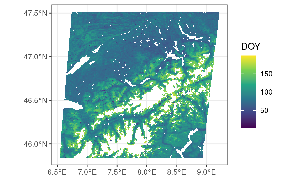
We can now compare both data sets in a spatially explicit way, e.g. compute overlap, reproject or resample data. For example, to limit computational time, it is often wise to restrict the region of interest to an overlapping section between both data sets. This allows data to be as large as required but as small as possible. We therefore crop the DEM data to correspond to the size of the coverage of the MODIS phenology data.
# crop the dem
dem <- terra::crop(
  x = dem,
  y = phenology_raster
)
The grid of the DEM and MODIS data do not align. Therefore, resampling of the data to a common grid is required. We use the grid of the highest resolution data as a template for this resampling, taking the average across the extent of a MODIS pixel.
# resample the dem using
# the mean DEM value in a
# MODIS pixel
dem <- terra::resample(
  x = dem,
  y = phenology_raster,
  method = "average"
)

# mask the locations which
# have no data
dem <- terra::mask(
  dem,
  is.na(phenology_raster),
  maskvalues = TRUE
)
To provide some context to our results, it might be useful to look at different responses by land cover class. In addition to phenology data, we can therefore also download the MODIS land cover data product for 2012.
# download and save land cover data
land_cover <- MODISTools::mt_subset(
  product = "MCD12Q1",
  lat = 46.6756,
  lon = 7.85480,
  band = "LC_Type1",
  start = "2012-01-01",
  end = "2012-12-31",
  km_lr = 100,
  km_ab = 100,
  site_name = "swiss",
  internal = TRUE,
  progress = FALSE
)
Now, convert this data to a geospatial format as before.
land_cover_raster <- MODISTools::mt_to_terra(
  land_cover,
  reproject = TRUE
)
4.3 Phenology trends
With all data processed, we can explore some of the trends in phenology in relation to topography. Plotting the data side by side already provides some insight into expected trends.
Code
p <- ggplot() +
  tidyterra::geom_spatraster(data = dem) +
  scale_fill_viridis_c(
    na.value = NA,
    name = "altitude (m)"
    ) +
  theme_bw()

p2 <- ggplot() +
  tidyterra::geom_spatraster(data = phenology_raster) +
  scale_fill_viridis_c(
    na.value = NA,
    name = "DOY"
    ) +
  theme_bw()

# compositing with patchwork package
library(patchwork)
p + p2 +
  plot_layout(ncol = 1) +
  plot_annotation(
    tag_levels = "a",
    tag_prefix = "(",
    tag_suffix = ")"
    )
We can plot the relation between topography and the start of the season (phenology) across the scene (where data is available). Plotting this non-spatially will show a clear relation between topography (altitude) and the start of the season. With an increasing altitude, we see the start of the season being delayed. The effect is mild below 1000m and increases above this.
Code
# convert to data frame and merge
dem_df <- as.vector(dem)
phenology_df <- as.vector(phenology_raster)
sct_df <- data.frame(
  altitude = dem_df,
  doy = phenology_df
  )

ggplot(
  data = sct_df,
      aes(
      altitude,
      doy
    )
  ) +
  geom_hex() +
  scale_fill_viridis_c(trans="log10") +
  geom_smooth(
    method = "lm",
    se = FALSE,
    colour = "white",
    lty = 2
  ) +
  labs(
    x = "altitude (m)",
    y = "MODIS vegetation greenup (DOY)"
  ) +
  theme_bw()
NoteNote
The fit linear regression above has the following parameters.
# fit a linear regression to the data of the figure above
# (for the pre-processing see the collapsed code of the figure)
fit <- lm(doy ~ altitude, data = sct_df)
print(summary(fit))
Call:
lm(formula = doy ~ altitude, data = sct_df)

Residuals:
     Min       1Q   Median       3Q      Max
-154.235   -8.431    0.092    9.426   78.967

Coefficients:
             Estimate Std. Error t value Pr(>|t|)
(Intercept) 5.421e+01  8.691e-02   623.7   <2e-16 ***
altitude    3.717e-02  6.915e-05   537.6   <2e-16 ***
---
Signif. codes:  0 '***' 0.001 '**' 0.01 '*' 0.05 '.' 0.1 ' ' 1

Residual standard error: 15.74 on 145522 degrees of freedom
  (44020 observations deleted due to missingness)
Multiple R-squared:  0.6651,    Adjusted R-squared:  0.6651
F-statistic: 2.89e+05 on 1 and 145522 DF,  p-value: < 2.2e-16