5  Phenology algorithms

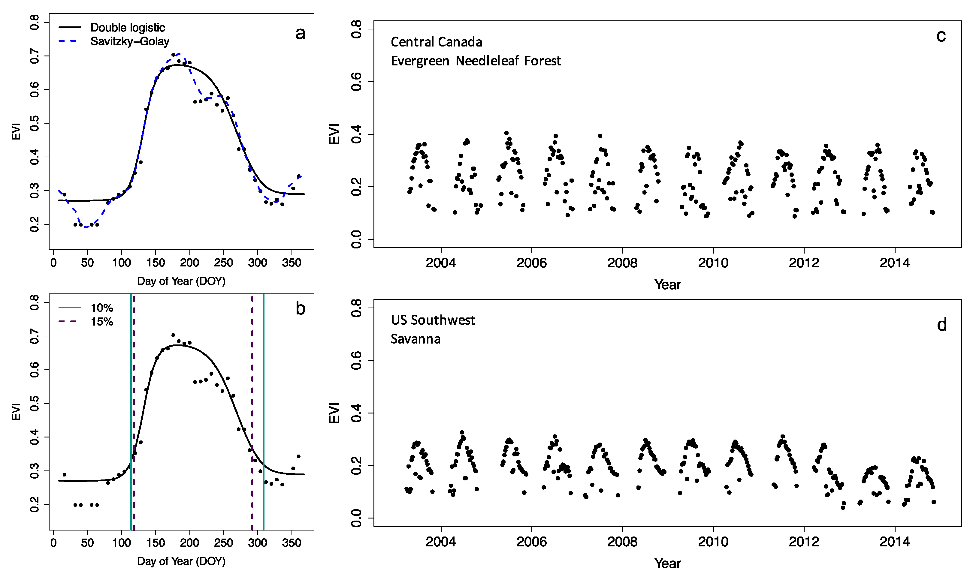
The example above, illustrating Hopkin’s law and the explicit temperature sensitivity of vegetation phenology to temperature, shows the importance of monitoring these changes within the context of climate change. In the previous example, we have used an operational land surface vegetation phenology data product.

Many products exist, depending on the remote sensing platform or data used, and cover a wide range of spatial scales. For example, the HR-VPP product allows for continuous vegetation monitoring using 10 m resolution Sentinel-2 data, while the previous example relies on 500 m resolution MODIS data. While MODIS provides a landscape-wide measure of vegetation phenology, the spatial scale of Sentinel-2 and its near real time data availability (low latency) allows for fine-grained assessments of crop growth.

5.1 Algorithms

5.1.1 Vegetation indices and time series

Most phenology data products rely on a limited set of algorithms, or various iterations of them, operating on time series of vegetation indices (VI), which combines various spectral bands (Figure 5.1) to provide information on vegetation status. Throughout the scientific literature, we can divide most methods for detection of phenological dates used in two categories:

• curve fitting
• threshold-based methods

The curve fitting approach fits a prescribed model structure to the data, by varying a number of parameters. This functional description of the vegetation growth can then be used to derive phenology metrics by considering various inflection points of this function. Common approaches are to use the first or second derivative of a fitted function (and zero crossings) to determine the timing of the most rapid change in vegetation phenology.

Figure 5.1: Example of a threshold-based phenology algorithm, by Stanimorova et al. 2019

The simplest approach, used with or without explicit curve-fitting, is the use of a simple threshold-based method. Here, a phenology event is registered if a given vegetation index threshold is crossed (Figure 5.1). Although scaling these products for global coverage is challenging, creating your own algorithm and implementing it on a local or regional scale is fairly simple. Below, it will be demonstrated how to calculate phenology for a vegetation index time series, for the region outlined in Chapter 4 .

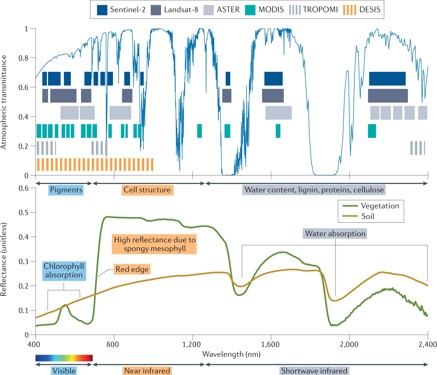
These methods are mostly applied to various vegetation indices, which link spectral characteristics as measured by satellites to the physical development of the canopy (Myneni et al. 1995; Huete et al. 2002). For example, the Normalized Vegetation Index (NDVI) uses both the red and near-infrared spectral domain (Figure 5.2) to sense the state of the vegetation, while the Enhanced Vegetation Index (EVI, Figure 5.1) does the same while accounting for the saturation of the signal over dense canopies. This multi-spectral nature of satellite remote sensing data, as well as their temporal dynamics, can be leveraged using a veritable zoo of indices tailored to specific properties and research needs (Zeng et al. 2022). An in-depth analysis on how to use these multi-spectral data in a different context is given in Chapter 7 .

Note

Given the non-continuous nature of the spectral bands used on most satellite platforms one calls these kinds of data multi-spectral. This in contrast to hyperspectral data which is quasi-continuous throughout a large spectral domain (Figure 5.2).

Figure 5.2: Figure from Zeng et al. (2022): ‘Satellite sensors, the vegetation and the soil spectrum across wavelengths. Top: the spectral response range in the atmospheric window of a few widely used satellites109. The coloured blocks and vertical lines illustrate the spectral band range or bandpass for each satellite sensor. Bottom: reflectance of vegetation and soil. These spectral features of vegetation and soil are the foundation of the rationale of vegetation indices and support the design of various vegetation indices.’ (if no image is shown you do not have institutional access to the original article content)

5.1.2 Acquiring demo data

To get started we need to download some additional information, in particular vegetation time series. In this example, and to lighten the download requirements, I will use Leaf Area Index (LAI) data instead of the more common EVI or NDVI time series used in phenology products. This is a pragmatic decision, based upon the availability of data.

# download data
df <- MODISTools::mt_subset(
  product = "MCD15A3H",
  lat = 42.536669726040884,
  lon = -72.17951595626516,
  band = "Lai_500m",
  start = "2002-01-01",
  end = "2022-12-31",
  km_lr = 0,
  km_ab = 0,
  site_name = "HF",
  internal = TRUE,
  progress = TRUE
)

5.2 Data quality control

Many data products have data quality flags, which allow you to screen your data for spurious values. However, in this example I will skip this step as the interpretation/use of these quality control flags is rather complex. The below methodology is therefore a toy example and further developing this algorithm would require taking into account these quality control metrics. Instead a general smoothing of the data will be applied.

5.3 Data smoothing and interpolation

We first multiply the data with their required scaling factor, transform the date values to a formal date format, and extract the individual year from the date.

# convert dates to proper date formats and
# convert the date to a single year
df <- df |>
  mutate(
    # scale the values correctly
    value =  value * as.numeric(scale),
    date = as.Date(calendar_date),
    year = as.numeric(format(date, "%Y")) 
  )

Smoothing can be achieved using various algorithms, such as splines, LOESS regressions, and other techniques. In this case, I will use the Savitsky-Golay filter, a common algorithm used across various vegetation phenology products. Luckily the methodology is already implemented in the signal package.

# load the signal library
library(signal)

# smooth this original input data using a
# savitski-golay filter
df <- df |>
  mutate(
    smooth = signal::sgolayfilt(value, p = 3, n = 31)
  )

Note that the sgolayfilt() does not allow for NA values to be present to function properly. Therefore, we operate on the full data set at its original time step. Since data is only provided at a 8-day time interval, you would be limited to this time resolution in determining final phenology metrics when using a threshold-based approach.

To get estimates close to a daily time step, we need to expand the data to a daily time-step and merge the original smoothed data.

# expand the time series to a daily time step
# and merge with the original data
expanded_df <- dplyr::tibble(
  date = seq.Date(min(df$date), max(df$date), by = 1)
)

# join the expanded series with the
# original data
df <- dplyr::left_join(expanded_df, df)

# back fill the year column for later
# processing
df <- df |>
  mutate(
    year = as.numeric(format(date, "%Y"))
  )

Expanding the 8-day data to a 1-day timestep will result in NA values. I will use a simple linear interpolation between smoothed 8-day values to acquire a complete time series without gaps.

# non NA values
no_na <- which(!is.na(df$smooth))

# finally interpolate the expanded dataset
# (fill in NA values)
df$smooth_int <- signal::interp1(
  x = as.numeric(df$date[no_na]),
  y = df$smooth[no_na],
  xi = as.numeric(df$date),
  method = 'linear'
)

Code

ggplot(df) +
  geom_point(
    aes(
      date,
      value
    ),
    colour = "red"
  ) +
  geom_line(
    aes(
      date,
      smooth_int
    )
  ) +
  labs(
    x = "",
    y = "LAI"
  ) +
  xlim(
    c(
    as.Date("2003-01-01"),
    as.Date("2005-12-31")
    )
  ) +
  theme_bw()

Figure 5.3: Smoothed LAI values as a black line, with original values as red circles

5.4 Phenology estimation

With all data prepared we can use an arbitrary threshold to estimate a transition in LAI values for a given year. In the example below, we use a LAI value of 3 to mark if the season has started or ended. To show the response to heterogeneous time series, I halved the values for the year 2004.

# half the values for 2004
# to introduce heterogeneity
df <- df |>
  mutate(
    smooth_int = ifelse(
      year == 2004,
      smooth_int/2,
      smooth_int
    )
  )

# calculate phenology dates on
# the smoothed time series
phenology <- df |>
  group_by(year) |>
  summarize(
    SOS = date[which(smooth_int > 3)][1],
    EOS = last(date[which(smooth_int > 3)])
  )

Code

ggplot(df) +
  geom_point(
    aes(
      date,
      value
    ),
    colour = "red"
  ) +
  geom_line(
    aes(
      date,
      smooth_int
    )
  ) +
  labs(
    x = "",
    y = "LAI"
  ) +
  xlim(
    c(
    as.Date("2003-01-01"),
    as.Date("2005-12-31")
    )
  ) +
  geom_hline(
    aes(yintercept = 3),
    lty = 2
  ) +
  geom_vline(
    data = phenology,
    aes(xintercept = EOS)
  ) +
  geom_vline(
    data = phenology,
    aes(xintercept = SOS)
  ) +
  theme_bw()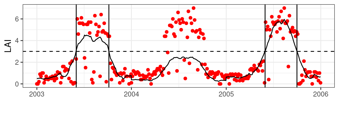

Figure 5.4: Calculated phenology dates using a fixed LAI threshold value, where the year 2004 smoothed values are artificially lowered. Smoothed LAI values as a black line, with original values as red circles. Vertical lines indicate the date when the yearly amplitude threshold of an LAI of 3 is exceeded. The dashed horizontal line illustrates that the lowered smoothed response does not meet any threshold requirement and shows no phenology response.

Obviously, this does not translate well to other locations, when vegetation types and densities vary from place to place. This is illustrated in Figure 5.4, using an artificially lowered signal in the year 2004, where years not meeting the absolute threshold will not produce accurate phenology estimates. Scaling the time series between 0 and 1 will regularize responses across time series and years and resolves this issue.

# potential issues?
# - fixed LAI threshold (varies per vegetation type)
# - does not account for incomplete years
# - provides absolute dates (not always helpful)
df <- df |>
  group_by(year) |>
  mutate(
    smooth_int_scaled = scales::rescale(
      smooth_int,
      to = c(0,1)
    )
  )

Now, we can use a relative amplitude (0 - 1) across locations and years. This ensures a consistent interpretation of what phenology represents. In case of a threshold of 0.5, this would represent the halfway point between a winter baseline and a summer maximum (leaf development) of a specific year and location. Commonly, one uses multiple thresholds to characterize different phases of the vegetation development. For example, a low threshold (~0.25) characterizes the start of the growing season, while a higher (~0.85) threshold marks the end of vegetation development toward summer.

As before, we can now apply relative thresholds (of 0.25 and 0.85) to our time series to mark the start of the season (SOS) and the maximum crown development (MAX). We can reverse this logic and use the same thresholds on the latter part of the seasonal trajectory and calculate the start of leaf senesence (SEN) and full leaf loss, or the end-of-season (EOS).

# calculate phenology dates
# SOS: start of season (25%, start)
# MAX: max canopy development (85%, start)
# SEN: canopy sensesence (85%, end)
# EOS: end of season (25%, end)
phenology <- df |>
  group_by(year) |>
  summarize(
    SOS = date[which(smooth_int_scaled > 0.25)][1],
    MAX = date[which(smooth_int_scaled > 0.85)][1],
    SEN = last(date[which(smooth_int_scaled > 0.85)]),
    EOS = last(date[which(smooth_int_scaled > 0.25)])
  )

Plotting these results for a limited set of years shows phenology dates for different years and phenology metrics (thresholds). Note that using the scaled (yearly) data estimates for the year 2004 yield robust phenology dates in spite of the artefactual multiplicative scaling that was introduced. This is in contrast to previous results as shown in Figure 5.4.

Code

ggplot(df) +
  geom_point(
    aes(
      date,
      value
    ),
    colour = "red"
  ) +
  geom_line(
    aes(
      date,
      smooth_int
    )
  ) +
  labs(
    x = "",
    y = "LAI"
  ) +
  xlim(
    c(
    as.Date("2003-01-01"),
    as.Date("2005-12-31")
    )
  ) +
  geom_vline(
    data = phenology,
    aes(xintercept = SOS),
    colour = "lightgreen"
  ) +
  geom_vline(
    data = phenology,
    aes(xintercept = MAX),
    colour = "darkgreen"
  ) +
  geom_vline(
    data = phenology,
    aes(xintercept = SEN),
    colour = "brown"
  ) +
  geom_vline(
    data = phenology,
    aes(xintercept = EOS),
    colour = "grey"
  ) +
  theme_bw()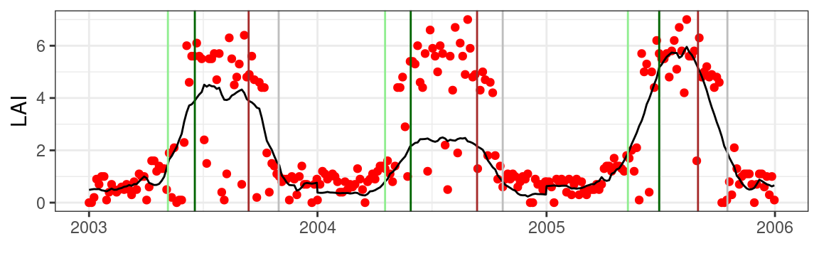

Figure 5.5: Calculated phenology dates using a fixed LAI threshold value, where the year 2004 smoothed values are artificially lowered. Smoothed LAI values as a black line, with original values as red circles. Vertical lines indicate the date when the yearly relative amplitude thresholds are exceeded. Light green indicates the start-of-season (SOS), dark green maximum canopy development (MAX), brown the start of senesence (SEN) and grey the end of season (EOS).

5.4.1 Spatial phenology estimates

The above example introduced the very basics of how to deal with a simple time series and develop a proof of concept. However, to scale our example spatially you need a way to process data along space and time axis. As introduced earlier, the terra package allows you to manipulate 3D data cubes (along latitude, longitude, and time axis).

# Download a larger data cube
# note that I sample a 100x100 km
# area around the lat/lon location
lai_2012 <- MODISTools::mt_subset(
  product = "MCD15A3H",
  lat = 46.6756,
  lon = 7.85480,
  band = "Lai_500m",
  start = "2012-01-01",
  end = "2012-12-31",
  km_lr = 100,
  km_ab = 100,
  site_name = "swiss",
  internal = TRUE,
  progress = TRUE
)

# save this data for later use
# to speed up computation

However, data downloaded using MODISTools by default is formated as tidy (row oriented) data. We use the mt_to_terra() function to convert this tidy data to a terra raster object.

# conversion from tidy data to a raster format
r <- MODISTools::mt_to_terra(
  lai_2012,
  reproject = TRUE
  )

Remember the algorithm for a single time series above. To make this collection of steps re-usable within the context of a multi-layer terra raster object (or data cube) you need to define a function. This allows you to run the routine across several pixels (at once).

Below I wrap the steps as defined in Section 5.4 in a single function which takes a data frame as input, a phenological phase and threshold value (0 - 1) as parameters. For this example we set the parameter to 0.5, or half the seasonal amplitude.

phenophases <- function(
    df,
    return = "start",
    threshold = 0.5
) {

  # split out useful info
  value <- as.vector(df)
  
  # if all values are NA
  # return NA (missing data error trap)
  if(all(is.na(value))) {
    return(NA)
  }
  
  date <- as.Date(names(df))
  
  # pick n to be 1/3th the total length
  # of the time series (in recorded values)
  # n must be odd
  n <- 31
  
  # smooth this original input data using a
  # savitski-golay filter
  smooth <- try(signal::sgolayfilt(
    value,
    p = 3,
    n = n
    )
  )
  
  # expand the time series to a daily time step
  # and merge with the original data
  date_expanded <- seq.Date(min(date, na.rm = TRUE), max(date, na.rm = TRUE), by = 1)
  smooth_int <- rep(NA, length(date_expanded))
  smooth_int[which(date_expanded %in% date)] <- smooth

  # non NA values for interpolation
  no_na <- which(!is.na(smooth_int))
  
  # finally interpolate the expanded dataset
  # (fill in NA values)
  smooth_int <- signal::interp1(
    x = no_na,
    y = smooth_int[no_na],
    xi = 1:length(smooth_int),
    'linear'
  )

  # rescale values between 0 and 1
  smooth_int_scaled <- scales::rescale(
    smooth_int,
    to = c(0,1)
  )
  
  # thresholding for phenology detection
  phenophase <- ifelse(
    return == "start",
    date_expanded[
      which(smooth_int_scaled > threshold)
      ][1],
    last(
      date_expanded[
        which(smooth_int_scaled > threshold)
        ]
      )
  )

  # convert to doy
  doy <- as.numeric(format(as.Date(phenophase, origin = "1970-01-01"),"%j"))
  return(doy)
}

With the function defined we can now apply this function to all pixels, and along the time axis (layers) of our terra raster stack. The app() function allows you to do exactly this! You can now apply the above function to the time component (z-axis, i.e. various layers) of the LAI data cube.

# apply a function to the z-axis (time / layers) of a data cube
phenology_map <- app(r, phenophases)

The generated dynamic map Figure 5.6 shows the result of the algorithm and allows us to explore some of the underlying reasons for the observed patterns. For example, meadows and agricultural fields often show early leaf development, while forested areas exhibit later phenology dates. Our own new “product” shows differences with the MODIS (MCD12Q2) phenology product, which can be attributed to methodological choices.

Exercise

Think of the various ways the algorithm design could change the results relative to the algorithm used in the MODIS (MCD12Q2) phenology product.

Code

library(leaflet)

# set te colour scale manually
pal <- colorNumeric(
  "magma",
  values(phenology_map),
  na.color = "transparent"
  )

# build the leaflet map
# using ESRI tile servers
# and the loaded demo raster
leaflet() |> 
  addProviderTiles(providers$Esri.WorldImagery, group = "World Imagery") |>
  addProviderTiles(providers$Esri.WorldTopoMap, group = "World Topo") |>
  addRasterImage(
    phenology_map,
    colors = pal,
    opacity = 0.8,
    group = "Custom phenology"
    ) |>
  addRasterImage(
    phenology_raster,
    colors = pal,
    opacity = 1,
    group = "MODIS phenology"
    ) |>
  addLayersControl(
    baseGroups = c("World Imagery","World Topo"),
    position = "topleft",
    options = layersControlOptions(collapsed = FALSE),
    overlayGroups = c("Custom phenology","MODIS phenology")
    ) |>
  addLegend(
    pal = pal,
    values = values(phenology_map),
    title = "DOY")

Figure 5.6: Dynamic output of the generated phenology map. Toggle different layers to visualize the different products (MODIS or custom).

Note

The downloading of the Leaf Area Index data can be slow. If this process takes too long you can load the data from a pre-loaded online source:

https://github.com/geco-bern/handfull_of_pixels/raw/main/data/lai_2012.rds

# load RDS data using
r <- readRDS("url")

Huete, A, K Didan, T Miura, E P Rodriguez, X Gao, and L G Ferreira. 2002. “Overview of the Radiometric and Biophysical Performance of the MODIS Vegetation Indices.” Remote Sensing of Environment 83 (1-2): 195–213. citeulike-article-id:274524http://dx.doi.org/10.1016/S0034-4257(02)00096-2.

Myneni, RB, FG Hall, Piers J. Sellers, and Alexander L. Marshak. 1995. “The Interpretation of Spectral Vegetation Indexes.” Transactions on Geoscience and Remote Sensing 33 (2): 481–86. http://ieeexplore.ieee.org/xpls/abs_all.jsp?arnumber=377948.

Zeng, Yelu, Dalei Hao, Alfredo Huete, Benjamin Dechant, Joe Berry, Jing M. Chen, Joanna Joiner, et al. 2022. “Optical Vegetation Indices for Monitoring Terrestrial Ecosystems Globally.” Nature Reviews Earth & Environment 3 (7): 477–93. https://doi.org/10.1038/s43017-022-00298-5.