
7 Land-Cover classification
In previous sections I have explained how the timing in the development of vegetation canopy density (i.e. using the leaf area index, or LAI) can be detected, and how it varies depending on the geography of the region. I introduced how this ties to the exchange of carbon and water between the biosphere and the atmosphere (Chapter 4). A small, first principles, example was provided on how to write your own phenology detection algorithm (Chapter 5) and how to use such data to model phenology, based upon environmental drivers (Chapter 6). In this section I will cover Land-Use and Land-Cover classification and explain how all these concepts relate.
When we plot a time series of the LAI of a deciduous forest you note the steady seasonal changes when switching between winter, with low LAI values, to summer with high LAI values. However, different vegetation (and Land-Use and Land-Cover) types have different temporal LAI profiles. For example, a glacier will have permanent snow and no seasonal LAI signal. We can therefore discriminate (visually) between non-vegetative locations and vegetation based upon the combined spectral and temporal profiles across locations (Figure 7.1).
We can use this concept, of differential temporal and spectral responses to map where certain Land-Use and Land-Cover types are dominant. In the above example, I used LAI which is a derived index which uses raw spectral data and an underlying model. However, satellite platforms provide raw information in various spectral bands. One can say the data are multi-dimensional, having both a temporal, spatial and spectral component (see Figure 5.2). These various bands, or locations in the spectral domain, provide key insights into the state of the land surface (throughout the year). For example the combination of information in the red and near-infrared bands (spectral domains) provides key information to calculate the Normalized Difference Vegetation Index (NDVI) (Huete et al. 2002) an indicator of plant health and density. Other band combinations and or models lead to other indices, e.g. the LAI data previously used, with varying properties tailored to specific ecological, geo-morphological or other purposes (Zeng et al. 2022). All this spectral-temporal data combined with machine learning (clustering) approaches allows us to map the land surface in great detail. In this section I will discuss both unsupervised and supervised machine learning approaches to Land-Use and Land-Cover (LULC) mapping.
NoteNote
Land-Use and Land-Cover (LULC) mapping is often mentioned as one concept. However, it is important to note the difference between Land-Use and Land-Cover. Land-Use is determined by human activities, while Land-Cover is the consequence of the natural biotic and abiotic environment. Although in an age of climate change (and global rising CO2 levels and temperatures) few places are truly free of human influence this nuance remains noteworthy. In this chapter I will focus mostly on the Land-Cover aspect (the natural environment).
7.1 Unsupervised machine learning
Working of the concept as demonstrated in Figure 7.1 we can use the spectral and temporal information across the landscape to classify a Swiss alpine scene into locations which have little seasonality and those which have some. For example you can calculate the mean and standard deviation of a full year and see how much variability you see across a year. Regions with a low LAI signal with little variability are most likely not associated with vegetation (e.g. glaciers, see Figure 7.1). Classification of data in different classes (or clustering) can be accomplished using various methods. Clustering can either be unsupervised, where clustering is only defined by the number of classes one wants to divide the (multi-dimensional) dataset into, with no reference data to compare the results to.
In this example I use an unsupervised machine learning approach, called k-means clustering, to divide the dataset into two or more classes. These classes are clustered in a way which minimizes within-cluster variances, i.e. it ensures that pixels will look similar to each other (given a target number of clusters k to divide the dataset into).
Here, we can use the lai_2012 dataset we previously downloaded, but we’ll use the raster representation as a starting point (as most geospatial data will come in multi-layer raster formats).
# conversion from tidy data to a raster format
# as it is common to use raster data
r <- MODISTools::mt_to_terra(
  lai_2012,
  reproject = TRUE
  )
# load buffered data
# that is stored in the data folder of the repo
r <- terra::rast(here::here("../data/LAI.tiff"))As a first step (ironically) I will convert this raster object back into a dataframe, since this is the format expected by many machine learning packages. However, this time it will be a wide data frame, where every pixel location is a row and every column a value for a given date (see Chapter 1). Alternatively, I could have converted the original lai_2012 data frame from a long format into a wide format using tidyr::pivot_wider(). Every row, representing a year for a given location, is a feature (vector) which contains the information on which the k-means clustering algorithm will operate.
# convert a multi-layer raster image
# to wide dataframe
df <- as.data.frame(r, cell = TRUE)

# the content of a single feature (vector)
# limited to the first 5 values for brevity
print(df[1:3,1:5])
cell 2012-01-01 2012-01-05 2012-01-09 2012-01-13
43 43 0.6935470 1.309657 0.01870939 1.1064531
44 44 0.6387032 0.591392 0.01870939 0.8732780
45 45 0.5746563 0.000000 0.01241251 0.6602281We can now use the kmeans() algorithm to classify the data into two distinct groups or centers (k = 2). Note that we drop the first column from our dataframe as this contains the pixel indices, which are needed later on.
# cluster the data into k classes
clusters <- kmeans(
  df[,-1],     # -1 removes column 'cell'
  centers = 2  # setting k to 2
)
Finally, we map the cell values back onto those of the original extent of the LAI data (to retain their respective geographic position).
# use the original raster layout as
# a template for the new map (only
# using a single layer)
kmeans_map <- terra::rast(r, nlyr=1)

# assign to each cell value (location) of this
# new map using the previously exported cell
# values (NA values are omitted so a 1:1
# mapping would not work)
kmeans_map[df$cell] <- clusters$cluster
Code
library(leaflet)

# set te colour scale manually
palcol <- colorFactor(
  c("#78d203", "#f9ffa4"),
  domain = 1:2,
  na.color = "transparent"
  )

# build the leaflet map
leaflet() |>
  addProviderTiles(providers$Esri.WorldTopoMap, group = "World Topo") |>
  addProviderTiles(providers$Esri.WorldImagery, group = "World Imagery") |>
  addRasterImage(
    kmeans_map,
    colors = palcol,
    opacity = 0.5,
    method = "ngb",
    group = "k-means cluster results"
    ) |>
  addLayersControl(
    baseGroups = c("World Topo","World Imagery"),
    position = "topleft",
    options = layersControlOptions(collapsed = FALSE),
    overlayGroups = c("k-means cluster results")
    ) |>
  addLegend(
    colors = palcol(1:2),
    values = c(1, 2),
    title = "cluster",
    labels = c(1, 2)
)As the example uses an unsupervised classification we do not know what land cover types are included in this map. The model that we generate is therefore purely data informed, and not validated against external known Land-Use and Land-Cover locations. However, a quick visual inspection shows that for a k of 2 the split between the clusters divides vegetation from glaciers, water bodies, and urban areas (Figure 7.2). The (seasonal) differences in LAI were used in the k-means analysis to minimize the (seasonal) variance between pixels. In particular, our analysis with two classes separates areas with a seasonal dynamic from those without one. Although the k-means algorithm is fast it only has one parameter which can shape the outcome of algorithm (i.e. k). The model is therefore too inflexible for more complex classification tasks. Moreover, the k-means model is rarely used as a scalable solution to generate maps based upon in-situ reference labels. Approaches using reference labels are part of supervised machine learning (see example below).
In the above example I used a single index, i.e. LAI, which does not provide sufficient information to distinguish between more subtle Land-Use or Land-Cover classes (e.g. evergreen forests and or mixed forest types). In short, a better approach would use more data and a more sophisticated model approach to create an informed model which scales easily to different land cover types and new locations.
7.2 Supervised machine learning
In contrast to k-means, one can use supervised classification of data where reference data is used as labels on which to train a machine learning algorithm. A supervised machine learning algorithm will try to minimize the classification error on a known training or testing dataset. The methodology, model complexity and parameters are dependent on the provided data, the complexity of the problem and the available computational resources.
For example the creation of the MODIS land-cover and land-use product (MCD12Q2) uses >1500 reference locations, three years of temporal data and a variety of multiple spectral bands, as well as ancillary data (topography, view angle geometry) to train their boosted classification tree (Friedl et al. 2002, 2010). In the below example I will try to recreate a part of the MCD12Q2 LULC workflow (red boxes, Figure 7.3). A full introduction to machine learning is beyond the scope of this course and I refer to Boehmke and Greenwell (2020), Kuhn and Silge (2022) and the AGDS book for an introduction in machine learning using R.

7.2.1 Ground truth reference data
Critical in our exercise is the reference data we use to classify different Land-Use and Land-Cover types with. Generally ground truth data is used in order to create training and testing datasets. This ground truth data are locations which are visually validated to belong to a particular Land-Use or Land-Cover class. These data are gathered by in-situ surveys, or leverage high(er) resolution data and visual interpretation to confirm the the Land-Use or Land-Cover type.
For example, the LUCAS database of the European Commission Joint Research Center provides three-yearly survey data on the Land-Use and Land-Cover state (d’Andrimont et al. 2020), while the Geo-Wiki project used crowdsourcing to confirm Land-Use and Land-Cover types using high resolution remote sensing imagery (Fritz et al. 2017). Other products use in house databases using similar approaches (Friedl et al. 2010). In this example, I will rely on the freely available crowdsourced (Geo-Wiki) dataset (Fritz et al. 2017). These ground truth labels differ slightly from the International Geosphere-Biosphere Programme (IGBP) classes used in the MCD12Q1 product. Nevertheless, the general principles are the same.
# Read the reference (validation) sites from
# Fritz et al. 2017 straight from Zenodo.org
validation_sites <- readr::read_csv(
  "https://zenodo.org/record/6572482/files/Global%20LULC%20reference%20data%20.csv?download=1"
)
I will restrict the number of reference validation sites to a manageable number of 150 random locations for each Land-Use or Land-Cover class, limited to high quality locations on the northern hemisphere (as we will apply our analysis regionally to Switzerland). The ground truth data in Fritz et al. (2017) contains data from different crowdsourcing competitions. Nr. 1 refers to Land-Use and nr. 4 to Land-Cover classes. The below routine shows how to gather 150 random locations for each Land-Use or Land-Cover class from Fritz et al. (2017). The locations of this data will be used to train and test the supervised machine learning algorithm.
# filter out data by competition,
# coverage percentage and latitude
# (use round brackets to enclose complex
# logical statements in a filter call!)
validation_selection <- validation_sites |>
    dplyr::filter(
      (competition == 4 | competition == 1),
      perc1 > 80,
      lat > 0
    )

# the above selection includes all data
# but we now subsample to 150 random locations
# per (group_by()) land cover class (LC1)
# set a seed for reproducibilty
set.seed(0)

validation_selection <- validation_selection |>
    dplyr::slice_sample(n = 150, by = LC1)

# split reference selection
# by land cover type into a nested
# list, for easier processing
# later on
validation_selection <- validation_selection |>
    dplyr::group_by(LC1) |>
    dplyr::group_split()
validation_selection <- readr::read_rds(
here::here("data/competition_selection.rds")
);
# train and test data for the competition was
# downloaded with `data-raw/download_competition_data.R`
# and prepared with `data-raw/compile_training_data.R`
# (see https://github.com/geco-bern/handfull_of_pixels/)
# and deposited on Zenodo.
# see further below how to directly load train and
# test data (containing predictors and land-cover labels)
# from Zenodo. (Since this data is already prepared
# it is much quicker than the download with AppEEARS.)
NoteNote
The samples are generated randomly, although a random seed ensures some reproducibility it is wise to save your site selection on file.
7.2.2 Multi-spectral training data
As with our k-means clustering example we need predictor data to inform our supervised classification. The MODIS data product MCD43A4 provides daily multi-spectral data, which is corrected for (geometric) view angle effects between the satellite and the sun. In below example in the interest of time, we gather data for only four spectral bands (1 to 4) from the MCD43A4 data product. This is a subset of what is used in the formal MCD12Q1 LULC product.
The required MCD43A4 data is not readily available using the {MODISTools} R package, as previously introduced, and I will therefore rely on the {appears} R package (Hufkens 2023) to query and download training data. The {appears} package relies on the NASA AppEEARS API service which provides easy access to remote sensing data subsets similar to the ORNL DAAC service, as used by {MODISTools}. The provided data covers more data products, but does require a login (API key) limiting ad-hoc accessibility.
WarningWarning
I refer to the {appears} documentation for the setup and use of an API key. The instructions below assume you have registered and have a working key installed in your R session.
# for every row download the data for this
# location and the specified reflectance
# bands
task_nbar <- lapply(validation_selection, function(x){

  # loop over all list items (i.e. land cover classes)
  base_query <- x |>
    dplyr::rowwise() |>
    do({
      data.frame(
        task = paste0("nbar_lc_",.$LC1),
        subtask = as.character(.$pixelID),
        latitude = .$lat,
        longitude = .$lon,
        start = "2012-01-01",
        end = "2012-12-31",
        product = "MCD43A4.061",
        layer = paste0("Nadir_Reflectance_Band", 1:4)
      )
    }) |>
    dplyr::ungroup()

  # build a task JSON string
  task <- rs_build_task(
    df = base_query
  )

  # return task
  return(task)
})

# Query the appeears API and process
# data in batches - this function
# requires an active API session/login
rs_request_batch(
  request = task_nbar,
  workers = 10,
  user = "your_api_id",
  path = tempdir(),
  verbose = TRUE,
  time_out = 28800
)
# train and test data for the competition was
# downloaded with `data-raw/download_competition_data.R`
# and prepared with `data-raw/compile_training_data.R`
# (see https://github.com/geco-bern/handfull_of_pixels/)
# and deposited on Zenodo.
# see further below how to directly load train and
# test data (containing predictors and land-cover labels)
# from Zenodo. (Since this data is already prepared
# it is much quicker than the download with AppEEARS.)
NoteNote
AppEEARS downloads might take a while! In the code above the default directory is also set to the temporary directory. To use the above code make sure to change the download path to a more permanent one.
With both training and reference data downloaded we can now train a supervised machine learning model! We do have to wrangle the data into a format that is acceptable for machine learning tools. In particular, we need to convert the data from a long format to a wide format (see Section 1.4.1), where every row is a feature vector. The {vroom} package is used to efficiently read in a large amount of similar CSV files into a large dataframe using a single list of files (alternatively you can loop over and append files using base R).
# list all MCD43A4 files, note that
# that list.files() uses regular
# expressions. Thus when using wildcards
# such as *, you can use glob2rx() to
# convert these wildcards to regular
# expressions
files <- list.files(
  tempdir(),
  glob2rx("*MCD43A4-061-results*"),
  recursive = TRUE,
  full.names = TRUE
)

# read in the data (very fast)
# with {vroom} and set all
# fill values (>=32767) to NA
nbar <- vroom::vroom(files)
nbar[nbar >= 32767] <- NA

# retain the required data only
# and convert to a wide format
nbar_wide <- nbar |>
  dplyr::select(
    Category,
    ID,
    Date,
    Latitude,
    Longitude,
    starts_with("MCD43A4_061_Nadir")
  ) |>
  tidyr::pivot_wider(
    values_from = starts_with("MCD43A4_061_Nadir"),
    names_from = Date
  )

# split out only the site name,
# and land cover class from the
# selection of validation sites
# (this is a nested list so we
# bind_rows across the list)
sites <- validation_selection |>
  dplyr::bind_rows() |>
  dplyr::select(
    pixelID,
    LC1
  ) |>
  dplyr::rename(
    Category = "pixelID"
  )

# combine the NBAR and land-use
# land-cover labels by location
# id (Category)
ml_df <- left_join(nbar_wide, sites) |>
    dplyr::select(
    LC1,
    contains("band")
  )
# train and test data for the competition was
# downloaded with `data-raw/download_competition_data.R`
# and prepared with `data-raw/compile_training_data.R`
# (see https://github.com/geco-bern/handfull_of_pixels/)
# and deposited on Zenodo.
# see further below how to directly load train and
# test data (containing predictors and land-cover labels)
# from Zenodo. (Since this data is already prepared
# it is much quicker than the download with AppEEARS.)7.2.3 Model training
This example will try to follow the original MODIS MCD12Q1 workflow closely which calls for a boosted regression classification approach (Friedl et al. 2010). This method allows for the use of a combination of weak learners to be combined into a single robust ensemble classification models. The in depth discussion of the algorithm is beyond the scope of this course and I refer to specialized literature for more details. To properly evaluate or model we need to split our data in a true training dataset, and a test dataset. The test dataset will be used in the final model evaluation, where samples are independent of those contained within the training dataset (Boehmke and Greenwell 2020).
# select packages
# avoiding tidy catch alls
library(rsample)

# create a data split across
# land cover classes
ml_df_split <- ml_df |>
  rsample::initial_split(
  strata = LC1,
  prop = 0.8
)

# select training and testing
# data based on this split
train <- rsample::training(ml_df_split)
test <- rsample::testing(ml_df_split)
# train and test data for the competition was
# downloaded with `data-raw/download_competition_data.R`
# and prepared with `data-raw/compile_training_data.R`
# (see https://github.com/geco-bern/handfull_of_pixels/)
# and deposited on Zenodo.
# see here how to directly load train and test data from Zenodo
download.file(
url = "https://zenodo.org/records/8298491/files/test_data.rds?download=1",
destfile = file.path(tempdir(), "test_data.rds"))
download.file(
url = "https://zenodo.org/records/8298491/files/training_data.rds?download=1",
destfile = file.path(tempdir(), "training_data.rds"))
test_data_Zenodo <- readr::read_rds(
file.path(tempdir(), "test_data.rds"))
training_data_Zenodo <- readr::read_rds(
file.path(tempdir(), "training_data.rds"))
# ensure training and test data contain same predictor/feature variables
setdiff(names(training_data_Zenodo),
names(test_data_Zenodo)) # pixelID, LC1, lat, lon
setdiff(names(test_data_Zenodo),
names(training_data_Zenodo))
train <- training_data_Zenodo |>
select(-c(pixelID, lat, lon)) # remove ID, lat, lon
test <- test_data_Zenodo
# NOTE: for the competition, column 'LC1' was removed from the
# test dataWith both a true training and testing dataset in place we can start to implement our supervised machine learning model. I will use a “tidy” machine learning modelling approach. Similar to the data management practices described in Chapter 1, a tidy modelling approach relies mostly on sentence like commands using a pipe (|>) and workflows (recipes). This makes formulating models and their evaluation more intuitive for many. For an in depth discussion on tidy modelling in R I refer to Kuhn and Silge (2022). Now, let’s get started.
Model structure and workflow
To specify our model I will use the {parsnip} R package which goal it is “… to provide a tidy, unified interface to models that can be used to try a range of models without getting bogged down in the syntactical minutiae of the underlying packages”. Parsnip therefore will remove some of the complexity of using a package such as {xgboost} might present. It also allows you to switch between different model structures with ease, only swapping a few arguments. Parsnip will make sure that model parameters are correctly populated and forwarded.
Following (Friedl et al. 2010) we will implement a boosted regression (classification) tree using the {xgboost} R package, via the convenient {parsnip} R package interface. The model allows for a number of hyper-parameters, i.e. parameters which do not define the base {xgboost} algorithm but the implementation and structure of it. In this example hyper-parameters for the number of trees is fixed at 50, while the tree depth is flexible (parameters marked tune(), see below).
NoteNote
There are many more hyper-parameters. For brevity and speed these are kept at a minimum. However, model performance might increase when tuning hyper-parameters more extensively.
# load the parsnip package
# for tidy machine learning
# modelling and workflows
# to manage workflows
library(parsnip)
library(workflows)

# specify our model structure
# the model to be used and the
# type of task we want to evaluate
model_settings <- parsnip::boost_tree(
  trees = 50,
  min_n = tune(),
  tree_depth = tune(),
  # learn_rate = tune()
  ) |>
  set_engine("xgboost") |>
  set_mode("classification")

# create a workflow compatible with
# the {tune} package which combines
# model settings with the desired
# model structure (data / formula)
xgb_workflow <- workflows::workflow() |>
  add_formula(as.factor(LC1) ~ .) |>
  add_model(model_settings)

print(xgb_workflow)
══ Workflow ════════════════════════════════════════════════════════════════════
Preprocessor: Formula
Model: boost_tree()
── Preprocessor ────────────────────────────────────────────────────────────────
as.factor(LC1) ~ .
── Model ───────────────────────────────────────────────────────────────────────
Boosted Tree Model Specification (classification)
Main Arguments:
trees = 50
min_n = tune()
tree_depth = tune()
Computational engine: xgboost Hyperparameter settings
To optimize our model we need to configure (tune) the hyper-parameters which were left variable in the model settings. How we select these hyper-parameters is determined by sampling a parameter space, defined in our example by latin hypercube sampling. The {dials} R package provides a “tidymodels” compatible functions to support building latin hypercubes for our parameter search. In this example, I use the extract_param_set_dials() function to automatically populate the latin hypercube sampling settings. However, these can be specified manually when needed.
# load the dials package
# responsible for (hyper) parameter
# sampling schemes to tune
# parameters (as extracted)
# from the model specifications
library(tune)
library(dials)

hp_settings <- dials::grid_latin_hypercube(
  tune::extract_parameter_set_dials(xgb_workflow),
  size = 3
)

print(hp_settings)
# A tibble: 3 × 2
min_n tree_depth
<int> <int>
1 11 4
2 37 10
3 25 15Parameter estimation and cross-validation
We can move on to the actual model calibration. To ensure robustness of our model (hyper-) parameters across the training dataset the code below also implements a cross-validation to rotate through our training data using different subsets. The below code tunes the model parameters across the cross-validation folds and returns all these results in one variable, xgb_results.
# set the folds (division into different)
# cross-validation training datasets
folds <- rsample::vfold_cv(train, v = 3)

# optimize the model (hyper) parameters
# using the:
# 1. workflow (i.e. model)
# 2. the cross-validation across training data
# 3. the (hyper) parameter specifications
# all data are saved for evaluation
xgb_results <- tune::tune_grid(
  xgb_workflow,
  resamples = folds,
  grid = hp_settings,
  control = tune::control_grid(save_pred = TRUE)
)
When the model is tuned across folds the results show varied model performance. In order to select the best model, according to a set metric, you can use the select_best() function (for a specific metric). This will extract the model hyperparameters for model training.
# select the best model based upon
# the root mean squared error
xgb_best <- tune::select_best(
  xgb_results,
  metric = "roc_auc"
  )

# cook up a model using finalize_workflow
# which takes workflow (model) specifications
# and combines it with optimal model
# parameters into a model workflow
xgb_best_hp <- tune::finalize_workflow(
  xgb_workflow,
  xgb_best
)

print(xgb_best_hp)
══ Workflow ════════════════════════════════════════════════════════════════════
Preprocessor: Formula
Model: boost_tree()
── Preprocessor ────────────────────────────────────────────────────────────────
as.factor(LC1) ~ .
── Model ───────────────────────────────────────────────────────────────────────
Boosted Tree Model Specification (classification)
Main Arguments:
trees = 50
min_n = 11
tree_depth = 5
Computational engine: xgboost However, the returned object does not specify the model structure. To combine both the model structure (workflow) with the optimal parameters we need to combine both. In short, we need to finalize_workflow() which combines the model workflow with the model parameters into a final functional model workflow with optimal hyper-parameters. Note that the resulting model workflow does not contain any tunable (tune()) fields as shown above! The selected model workflow, given our provided constrains on the hyperparamters, has 50 trees, has minimum 11 data points in a node (min_n) and a tree depth of 5. We will use this workflow to fit() a final training run (on all training data data, i.e. including parts of the data that were set apart for the cross-validation runs) with the chosen optimal hyper-parameters. This returns our final model which provides the desired (classification) results!
# train a final (best) model with optimal
# hyper-parameters
xgb_best_model <- fit(xgb_best_hp, train)
7.2.4 Model evaluation on test data
In machine learning model evaluation can be achieved in various ways and the standard exploration of the accuracy and variables of importance (and their relative contributions) to the model strength are beyond the scope of this example. I will only focus on the standard methodology and terminology as used in remote sensing and GIS fields.
Confusion matrix and metrics
In the case of Land-Use and Land-Cover mapping classifications results are often reported as an confusion matrix and their associated metrics. The confusion matrix tells us something about accuracy (as perceived by users or producers), while the overall accuracy and Kappa coefficient allow us to compare the accuracy across modelled (map) results.
In Table 7.1 a three class confusion matrix is shown with the model prediction in rows and the reference (real) classes in columns. In addition, the user and producer accuracies are shown. The user accuracy is the fraction of correctly predicted classes with respect to the false positives (Type I) errors for a given prediction class. The producer accuracy is the fraction of correctly predicted classes with respect to the false negatives (Type II) errors for a given reference class.
| Ref. 1 | Ref. 2 | Ref. 3 | total | User accuracy (Type I) | Kappa | |
|---|---|---|---|---|---|---|
| Pred. 1 | 49 | 4 | 4 | 57 | 0.89 | |
| Pred. 2 | 2 | 40 | 2 | 44 | 0.90 | |
| Pred. 3 | 3 | 3 | 59 | 65 | 0.90 | |
| total | 54 | 47 | 65 | 166 | ||
| Producer accuracy (Type II) | 0.90 | 0.85 | 0.90 | 0.89 | ||
| Kappa | 0.84 |
NoteNote
In other words:
User accuracy: For example, among the sites that were predicted as class one (1) (first row) some were actually class two or three (2,3). The model committed the wrong label (1) to these sites. These false positives are therefore also called commission errors. Imagine a user of a prediction map is interested in a specific pixel that was predicted as class one (1), the user accuracy thus estimates how accurate this attribution to class one is.
Producer accuracy: Similarly, imagine a producer of a prediction map. Unlike the user, the producer has access to the reference data and wonders e.g. for all reference points of class one (1) (first column), how many got predicted correctly. For example, for all sites identified as class 1 in the reference data, some were predicted as class 2 and 3 by the model. These sites were omitted from the correct class and are thus also called omission errors.
In short, in remote sensing, the Type I and II errors are rephrased as the perspective taken during the assessment, either the user or the producer. In a strict machine learning context the user and producer accuracy would be called precision and recall, respectively. I refer to Boehmke and Greenwell (2020), Kuhn and Silge (2022) and the AGDS book for an in depth discussion on machine learning model evaluation. Also these online answers ([1], [2]) additionally explain the kappa statistic.
Simple confusion matrices can be calculated using R using the table() function comparing the true reference labels with the predicted values for our model. Using the function caret::confusionMatrix() gives directly additional overall- and by-class- statistics as shown below:
# run the model on our test data
# using predict()
test_results <- predict(xgb_best_model, test)

# load the caret library to
# access confusionMatrix functionality
library(caret)

# use caret's confusionMatrix function to get
# a full overview of metrics
caret::confusionMatrix(
  reference = as.factor(test$LC1),
  data = as.factor(test_results$.pred_class)
  )
Confusion Matrix and Statistics
Reference
Prediction 1 2 3 4 5 6 7 8 9 10
1 26 8 4 2 4 2 2 2 0 3
2 8 9 8 5 7 1 2 1 1 2
3 0 4 8 2 4 4 4 0 5 1
4 6 2 11 21 13 0 7 1 2 1
5 11 7 7 8 27 0 8 0 3 3
6 10 7 6 1 1 34 1 2 1 9
7 3 5 4 11 4 1 29 1 2 1
8 1 2 1 1 1 4 3 44 3 4
9 2 7 8 4 4 4 2 5 36 1
10 3 1 1 0 0 8 6 2 1 41
Overall Statistics
Accuracy : 0.4583
95% CI : (0.4179, 0.4992)
No Information Rate : 0.1167
P-Value [Acc > NIR] : < 2e-16
Kappa : 0.398
Mcnemar's Test P-Value : 0.07445
Statistics by Class:
Class: 1 Class: 2 Class: 3 Class: 4 Class: 5 Class: 6
Sensitivity 0.37143 0.17308 0.13793 0.38182 0.4154 0.58621
Specificity 0.94906 0.93613 0.95572 0.92110 0.9121 0.92989
Pos Pred Value 0.49057 0.20455 0.25000 0.32813 0.3649 0.47222
Neg Pred Value 0.91956 0.92266 0.91197 0.93657 0.9278 0.95455
Prevalence 0.11667 0.08667 0.09667 0.09167 0.1083 0.09667
Detection Rate 0.04333 0.01500 0.01333 0.03500 0.0450 0.05667
Detection Prevalence 0.08833 0.07333 0.05333 0.10667 0.1233 0.12000
Balanced Accuracy 0.66024 0.55460 0.54683 0.65146 0.6638 0.75805
Class: 7 Class: 8 Class: 9 Class: 10
Sensitivity 0.45312 0.75862 0.6667 0.62121
Specificity 0.94030 0.96310 0.9322 0.95880
Pos Pred Value 0.47541 0.68750 0.4932 0.65079
Neg Pred Value 0.93506 0.97388 0.9658 0.95345
Prevalence 0.10667 0.09667 0.0900 0.11000
Detection Rate 0.04833 0.07333 0.0600 0.06833
Detection Prevalence 0.10167 0.10667 0.1217 0.10500
Balanced Accuracy 0.69671 0.86086 0.7995 0.79001# NOTE: for the competition column 'LC1' was removed from
# the test data. Thus you can't compute the scores
# yourself.
#
# Instead upload your predictions from your best
# model as a pull request to
# https://github.com/geco-bern/agds2_course.
#
# To do so:
# a) save your results as .*csv:
readr::write_csv(
x = dplyr::rename(test_results,
lulc_class = .pred_class),
file = "~/Desktop/username_results.csv")
# a) fork the repository 'agds2_course',
# b) add and commit your results as
# 'data/leaderboard/fall_2025/username_results.csv',
# c) and open a pull request (PR) from your forked
# repository to the main repository at
# 'geco-bern/agds2_course'.
#
# Your predictions will then be added to the the leader
# board on the course website at
# https://geco-bern.github.io/agds2_course/leaderboard_fall_2025.html7.2.5 Model scaling to raster data
To scale our new model to other locations, or regions we will below download additional data covering the region around Bern. The code below demonstrates how to download geospatial raster data with the {appeears} R package, rather than point data used during training. This data will then be used to run our previously trained model, and the results will be presented as a map. Since our workflow closely followed the first steps of the MODIS MCD12Q1 LULC map protocol we will compare our map to the final MODIS MCD12Q1 product. (Since we did not use exactly the same MODIS IGBP Land-Use and Land-Cover classes we need to perform some remapping before plotting.)
Data download
To scale our analysis spatially we need to download matching data, i.e. MODIS MCD43A4 NBAR data for bands 1 through 4, for a geographic regions. The {appeears} R package has an roi parameter which can take SpatRaster map data. Providing a SpatRaster map will match its extent to the AppEEARS query. I will use the map generated during our k-means clustering exercise as the input for building an API task. Alternatively, you can provide an extent yourself using a polygon, as specified using the {sf} R package (Section 3.1.2).
# We can define an appeears
# download task using a simple
# dataframe and a map from which
# an extent is extracted
task_df <- data.frame(
  task = "raster_download",
  subtask = "swiss",
  start = "2012-01-01",
  end = "2012-12-31",
  product = "MCD43A4.061",
  layer = paste0("Nadir_Reflectance_Band", 1:4)
)

# build the area based request/task
# using the extent of our previous
# kmeans map, export all results
# as geotiff (rather than netcdf)
task <- rs_build_task(
  df = task_df,
  roi = kmeans_map,
  format = "geotiff"
)

# request the task to be executed
# with results stored in a
# temporary location (can be changed)
rs_request(
  request = task,
  user = "your_api_id",
  transfer = TRUE,
  path = tempdir(),
  verbose = TRUE
)
NoteNote
AppEEARS downloads might take a while! In the code above the default directory is also set to the temporary directory. To use the above code make sure to change the download path to a more permanent one.
Model prediction
The downloaded data (by default in tempdir()) are a collection of geotiff files of NBAR reflectance bands and their matching quality control data. In this demonstration I will not process the more nuanced quality control flags. Therefore, I only list the reflectance files, and read in this list of geotiffs into a stack by calling rast().
files <- list.files(
  tempdir(),
  "*Reflectance*",
  recursive = TRUE,
  full.names = TRUE
)

# load this spatial data to run the model
# spatially
swiss_multispec_data <- terra::rast(files)
The model we created is specific when it comes to naming variables, i.e. the naming of the bands in our spatial data matters and has to match those of the model. Due to inconsistencies in the AppEEARS API one has to rename the band names ever so slightly.
# the model only works when variable names
# are consistent we therefore rename them
band_names <- data.frame(
  name = names(swiss_multispec_data)
) |>
  mutate(
    date = as.Date(substr(name, 40, 46), format = "%Y%j"),
    name = paste(substr(name, 1, 35), date, sep = "_"),
    name = gsub("\\.","_", name)
  )

# reassign the names of the terra image stack
names(swiss_multispec_data) <- band_names$name
With all band names in line with the expected variables in our model we can now scale it by using terra::predict(). This function is the {terra} R package equivalent of the predict() function for general statistical models. This function allows you to call a compatible model for SpatRaster data, by running it along the time/band axis of the raster stack. I ask for the model probabilities to be returned, as this gives a more granular overview of the model results (see type argument, Figure 7.4).
# return probabilities, where each class is
# associated with a layer in an image stack
# and the probabilities reflect the probabilities
# of the classification for said layer
lulc_probabilities <- terra::predict(
  swiss_multispec_data,
  xgb_best_model,
  type = "prob"
)
Code
ggplot() +
  tidyterra::geom_spatraster(data = lulc_probabilities) +
  scale_fill_viridis_c(
    na.value = NA,
    name = "Class probabilities",
    option = "magma"
    ) +
  scale_x_continuous(breaks = seq(-180, 180, 2)) +
  theme_bw() +
  theme(
    legend.position = "bottom"
    ) +
  facet_wrap(~lyr)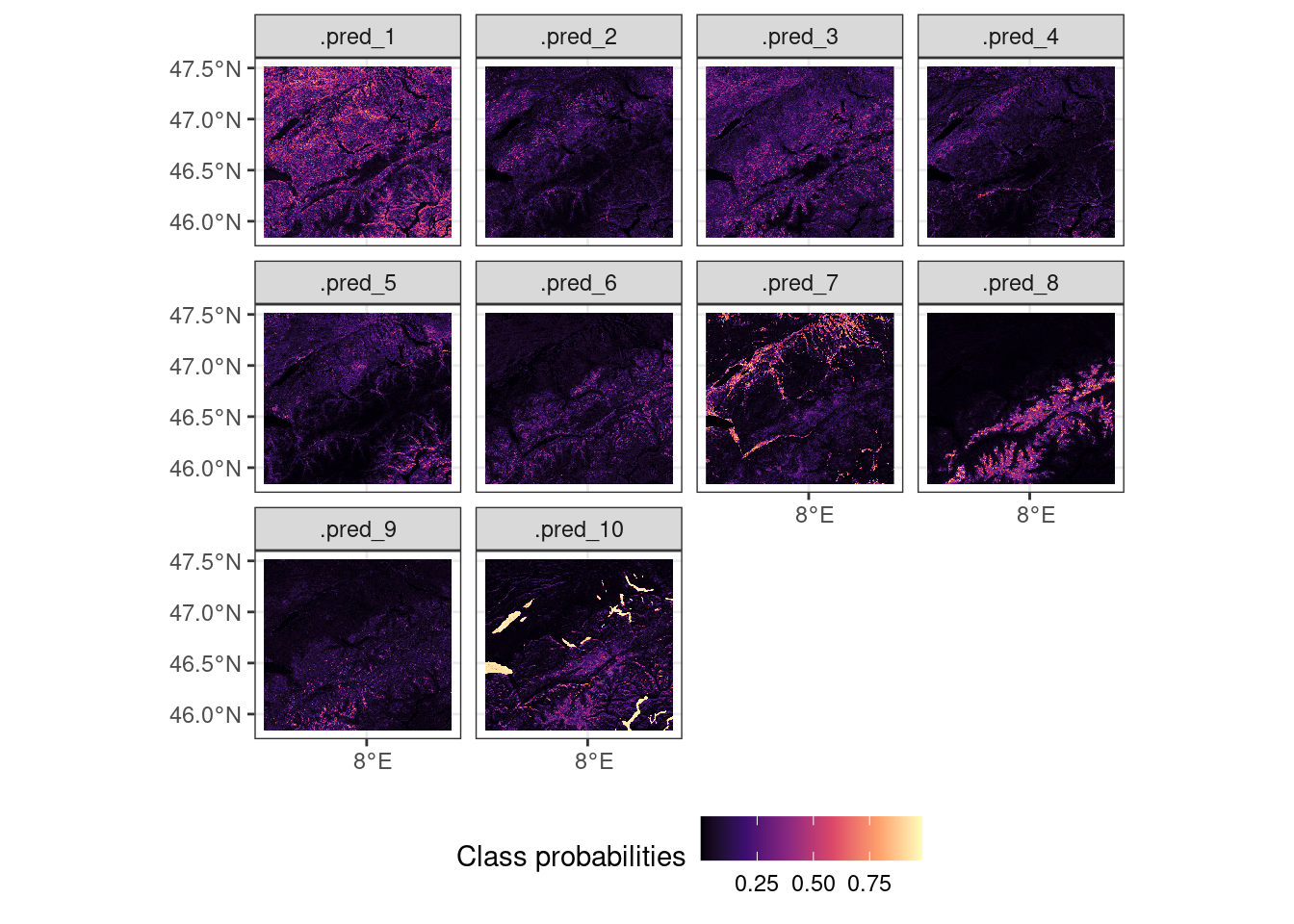
One can create a formal Land-Use and Land-Cover map by reducing this dataset by returning the layer for which the probability is highest, using which.max. As seen in Chapter 3, you can apply a function to all layers across pixels using the terra::app() function. The returned data is a Land-Use and Land-Cover map with classes 1 to 10, as shown below (Figure 7.5).
# generate the map by selecting maximum probabilities
# from the model output
lulc_map <- terra::app(lulc_probabilities, which.max)
Code
classes <- c(
    "Tree Cover",
    "Shrub Cover",
    "Herbaceous Vegetation & Grassland",
    "Cultivated and Managed",
    "Mosaic: Managed & Natural Vegetation",
    "Regularly Flooded & Wetland",
    "Urban & Built Up",
    "Snow and Ice",
    "Barren",
    "Open Water"
  )

# set te colour scale manually
palcol <- colorFactor(
  c(
    "#05450a",
    "#78d203",
    "#009900",
    "#c24f44",
    "#ff6d4c",
    "#27ff87",
    "#a5a5a5",
    "#69fff8",
    "#f9ffa4",
    "#1c0dff"
    ),
  na.color = NA,
  domain = 1:10
)

# build the leaflet map
leaflet() |>
  addProviderTiles(providers$Esri.WorldTopoMap, group = "World Topo") |>
  addProviderTiles(providers$Esri.WorldImagery, group = "World Imagery") |>
  addRasterImage(
    lulc_map,
    colors = palcol,
    opacity = 0.8,
    method = "ngb",
    group = "XGBOOST"
  ) |>
  addRasterImage(
    modis_lulc,
    colors = palcol,
    opacity = 0.8,
    method = "ngb",
    group = "MODIS MCD12Q1"
  ) |>
  addLayersControl(
    baseGroups = c("World Topo", "World Imagery"),
    position = "topleft",
    options = layersControlOptions(collapsed = FALSE),
    overlayGroups = c("XGBOOST", "MODIS MCD12Q1")
  ) |>
  hideGroup("MODIS MCD12Q1") |>
  addLegend(
    colors = palcol(1:10),
    values = 1:10,
    labels = classes,
    title = "Land-Use and Land-Cover class"
  )