Chapter 6 Open science practices
Chapter lead author: Koen Hufkens
6.1 Learning objectives
In this chapter, you will learn the reasons for practicing open science and some of the basic methodological techniques that we can use to facilitate an open science workflow.
In this chapter you will learn how to:
- structure a project
- manage a project workflow
- capture a session or machine state
- use dynamic reporting
- ensure data and code retention
6.2 Tutorial
The scientific method relies on repeated testing of a hypothesis. When dealing with data and formal analysis, one can reduce this problem to the question: could an independent scientist attain the same results given the described methodology, data and code?
Although this seems trivial, this issue has vexed the scientific community. These days, many scientific publications are based on complex analyses with often large data sets. More so, methods in publications are often insufficiently detailed to really capture the scope of an analysis. Even from a purely technical point of view, the reproducibility crisis or the inability to reproduce experimental results, is a complex problem. This is further compounded by social aspects and incentives. In recent decades, scientific research has seen a steady increase in speed due to the digitization of many fields and the commodification of science.
Although digitization has opened up new research possibilities, its potential for facilitating, accelerating, and advancing science are often not fully made use of. Historically, research and its output in the form of data and code has been confined to academic journals, data and code has often not been made available, and data were not shared or behind pay-walls. This limits the impact of science also in the public domain. (In many ways, this is still the case today, in year 2023 as we write). Digitization has made research output better visible and accessible, but practical obstacles and weak standards often prevent it from uptake, re-use, and further development by the wider community.
Open and reproducible science is a movement to make scientific research (output) widely accessible to the larger public, increase research transparency and enabling robust and verifiable science. Open science aims to be as open as possible about the whole scientific process, and as closed as desirable (e.g. privacy or security reasons).
It is important to acknowledge that there is a spectrum of reproducible data and code workflows which depends on the state or source of the data and the output of the code (or analysis). Within the context of this course, we focus primarily on the practical aspects for reproducible science, i.e., ensuring that given the same data and code, the results will be similar.
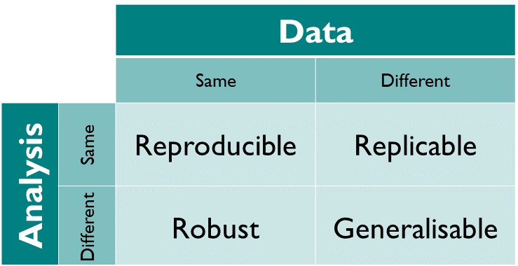
Figure 6.1: The reproducibility matrix by The Turing Way
The basics of open science coding and data practices rely on a number of simple concepts. The sections below describe a selection of the most important ones. Sticking to these principles and tools will increase the reproducibility of your work greatly.
6.2.1 Project structure
Reproducible science relies on a number of key components. Data and code management and the tracking of required meta-data is the first step in an open science workflow.
In Chapter 1, you learned how to setup an R project. An R project gathers all components of your analysis in a single directory. Although current computers make it easy to “find” your files and are largely file location-agnostic, this is not the case in many research environments. Projects grow quickly, and often, the number of files will flood a single directory. Therefore, files need a precise and structured location. This structure allows you to determine both the function and order of a workflow without reading any code.
It is good practice to have a consistent project structure within and between projects. This allows you to find most project components regardless of when you return to a particular project. Structuring a project in one folder also makes projects portable. All parts reside in one location making it easy to create a git project from this location (see Chapter 7), or just copy the project to a new drive.
An example data structure for raw data processing is given below and we provide an R project template to work from and adjust through our lab GitHub profile. A full description on using the template is provided in Chapter 7.
data-raw/
├─ raw_data_product/
├─ 00_download_raw_data.R
├─ 01_process_raw_data.R
6.2.2 Managing workflows
Although some code is agnostic to the order of execution, many projects are effectively workflows, where the output of one routine is required for the successful execution of the next routine.
In order to make sure that your future self, or a collaborator, understands the order in which things should be executed, it is best to number scripts accordingly. This is the most basic approach to managing workflows.
In the example below, all statistics code is stored in the statistics folder in an overall analysis folder (which also includes code for figures). All statistical analyses are numbered to ensure that the output of a first analysis is available to the subsequent one.
analysis/
├─ statistics/
│  ├─ 00_randomforest_model.R
│  ├─ 01_randomforest_tuning.R
├─ figures/
│  ├─ global_model_results_map.R
│  ├─ complex_process_visualization.R
The code-chunk above is a visualisation of a folder (aka. directory) structure on your computer. The lines and indents denote folder levels. In this example, you have a folder analysis which holds two more folders statistics and figures, and in both sub-folders, you have different *.R files (* is a so-called “wild-card” which is a placeholder for any text). Note that different people may use different symbols to visualise folder structures but generally, folder levels are shown with indents, and files are identifiable by their suffixes.
6.2.2.1 Automating and visualizing workflows with targets
To sidestep some of the manual management in R you can use a dedicated pipeline tool like the {targets} package in R. The package learns how your pipeline fits together, skips tasks that are already up-to-date, and runs only the necessary computation. {targets} can also visualize the progress of your workflow.
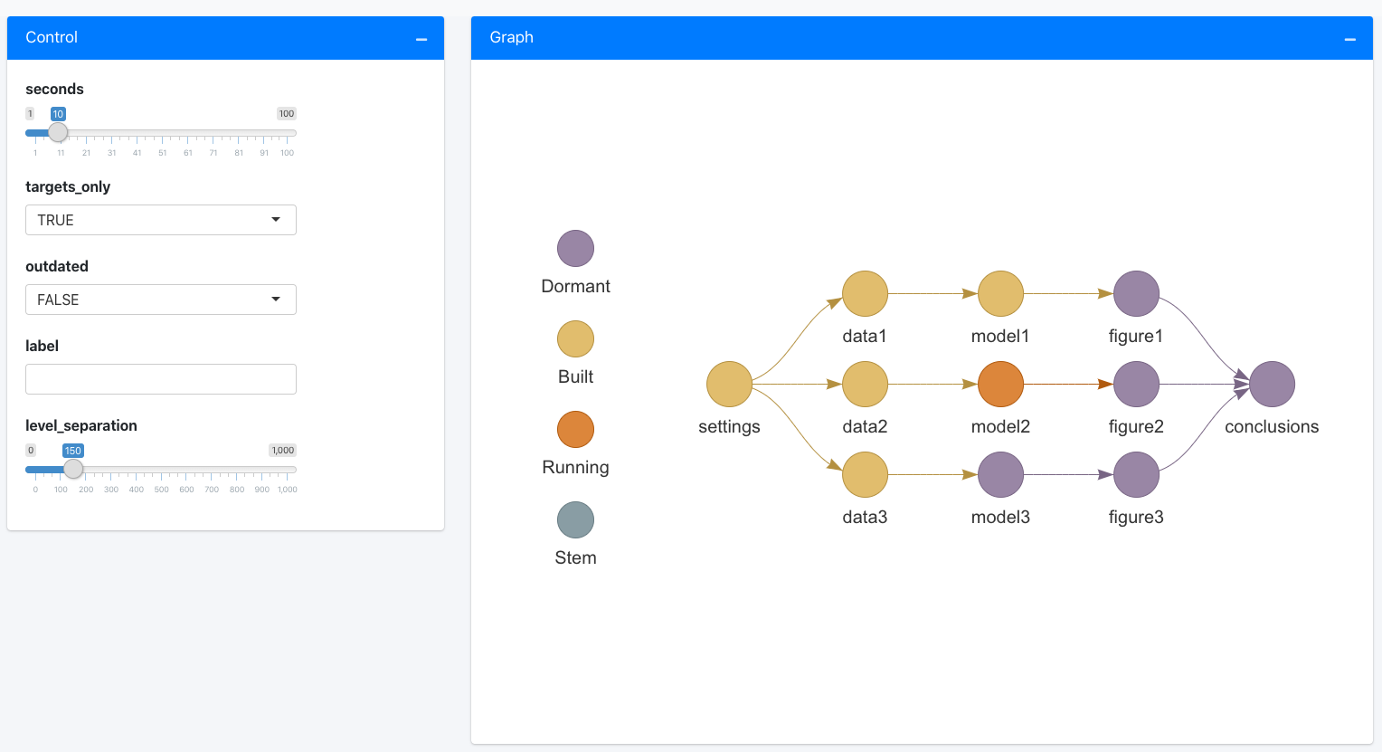
Figure 6.2: A targets visualized workflow by rOpenSci
Due to the added complexity of the {targets} package, we won’t include extensive examples of such a workflow but refer to the excellent documentation of the package for simple examples here.
6.2.3 Capturing your session state
Often, code depends on various components, packages or libraries. These libraries and all software come in specific versions, which might or might not alter the behaviour of the code and the output it produces.
If you want to ensure full reproducibility, especially across several years, you will need to capture the state of the system and libraries with which you ran the original analysis.
In R the {renv} package serves this purpose and will provide an index of all the packages used in your project as well as their version. For a particular project, it will create a local library of packages with a static version. These static packages will not be updated over time, and therefore ensure consistent results. This makes your analysis isolated, portable, and reproducible. The analogue in Python would be the virtual environments, or venv program.
When setting up your project you can run:
# Initiate a {renv} environment
renv::init()
To initiate your static R environment. Whenever you want to save the state of your project (and its packages) you can call:
# Save the current state of the environment / project
renv::snapshot()
To save any changes made to your environment. All data will be saved in a project description file called a lock file (i.e. renv.lock). It is advised to update the state of your project regularly, and in particular before closing a project.
When you move your project to a new system, or share a project on github with collaborators, you can revert to the original state of the analysis by calling:
# On a new system, or when inheriting a project
# from a collaborator you can use a lock file
# to restore the session/project state using
renv::restore()
NOTE: As mentioned in the {renv} documentation: “For development and collaboration, the
.Rprofile,renv.lockandrenv/activate.Rfiles should be committed to your version control system. But therenv/librarydirectory should normally be ignored. Note thatrenv::init()will attempt to write the requisite ignore statements to the project.gitignore.” We refer to 6.1 for details on github and its use.
6.2.4 Capturing a system state
Although R projects and the use of {targets} make your workflow consistent, the package versions used between various systems (e.g., your home computer or the cluster at the university might vary). To address issues with changes in the versions of package, you can use the {renv} package which manages package version (environments) for you. When tasks are even more complex and include components outside of R, you can use Docker to provide containerization of an operating system and the included ancillary application.
The {rocker} package provides access to some of these features within the context of reproducible R environments. Using these tools, you can therefore emulate the state of a machine, independently of the machine on which the docker file is run. These days, machine learning applications are often deployed as docker sessions to limit the complexity of installing required software components. The application of docker-based installs is outside the scope of the current course, but feel free to explore these resources as they are widespread in data science.
6.2.5 Readable reporting using Rmarkdown
Within Rstudio, you can use Rmarkdown dynamic documents to combine both text and code. Rmarkdown is ideal for reporting, i.e., writing your final document and presenting your analysis results. A Rmarkdown document consists of a header that specifies document properties (whether it should be rendered as an html page, a docx file or a pdf), and the actual content. You have encountered RMarkdown already in Chapter 1.2.6.
6.2.6 Project structure
In R projects, all files can be referenced relative to the top-most path of the project. When opening your_project.Rproj in RStudio, you can load data that is located in a sub-directory of the project directory ./data/ by read.table("./data/some_data.csv"). The use of relative paths and consistent directory structures across projects, enables that projects can easily be ported across computers and code adopted across projects.
project/
├─ your_project.Rproj
├─ vignettes/
│  ├─ your_dynamic_document.Rmd
├─ data/
│  ├─ some_data.csv
Rmarkdown files commonly reside in a sub-directory ./vignettes/ and are rendered relative to the file path where it is located. This means that to access data which resides in data/ using code in ./vignettes/your_dynamic_document.Rmd, we would have to write:
data <- read.table('../data/some_data.csv')Note the ../ to go one level up. To allow for more flexibility in file locations within your project folder, you may use the {here} package package. I gathers the absolute path of the R project and allows for a specification of paths inside scripts and functions that always start from the top project directory, irrespective of where the script that implements the reading-code is located. Therefore, we can just write:
data <- read.table(here::here('data/some_data.csv'))But why not use absolute paths to begin with? Portability! When I would run your \*.Rmd file with an absolute path on my computer, it would not render as the file some_data.csv would then be located at: /my_computer/project/data/some_data.csv
6.2.6.1 Limitations of notebooks
The file referencing issue and the common use of Rmarkdown, and notebooks in general, as a one size fits all solution, containing all aspects from data cleaning to reporting, implies some limitations. RMarkdown documents mix two cognitive tasks, writing text content (i.e. reporting) and writing code. Switching between these two modes comes with undue overhead. If you code, you should not be writing prose, and vise versa.
If your R markdown file contains more code than it does text, it should be considered an R script or function (with comments or documentation). Conversely, if your RMarkdown file contains more text than code, it probably is easier to collaborate on a true word processing file (or cloud-based solution). Notebooks, such as RMarkdown, are most suitable for communicating implementations, demonstrating functions, and reporting reproducible results. They can also be used like lab notes. They are less suited for code development.
6.2.7 Data retention
Coding practices and documenting all moving parts in a coding workflow is only one practical aspect of open science. An additional component is long-term data and code retention and versioning.
In Chapter 7, you will learn more about git for code management and collaboration. Several online make use of git for providing web-based collaboration functionalities and remote storage of your repositories. Examples are GitHub, GitLab, Codeberg, or Bitbucket. However, their remote storage service should only be considered an aid for collaboration, and not a place to store code into perpetuity. Furthermore, these services mostly have a limit to how much data can be stored in a repository (mostly ~2 GB). For small projects, data can be included in the repository itself. For larger projects and for making larger datasets accessible, this won’t be possible.
To ensure long-term storage of code and data, outside of commercial for profit services (e.g., Dropbox, Google Drive etc), it is best to rely on public permanent repositories, such as Zenodo. Zenodo is an effort by the European commission, but accessible to all, to facilitate archiving of science projects of all nature (code and data) up to 50 GB. In addition, Zenodo provides a citable digital object identifier or DOI. This allows data and code, even if not formally published in a journal, to be cited. Other noteworthy open science storage options include Dryad and the Center for Open Science.
The broad-purpose permanent data repositories mentioned above are not edited and are therefore not ideal for data discovery. In contrast, edited data repositories often have a specific thematic scope and different repositories are established in different research communities. Below you find a list of widely used data repositories, generalist and others, that provide manual or automated download access to their data. Note that this list contains some example and is far from extensive.
| Data type | Website | Description | Download |
|---|---|---|---|
| Copernicus Climate Data Store | https://cds.climate.copernicus.eu | Freely available climate data (reanalysis as well as future projections) | API |
| Oak Ridge National Laboratories Digital Active Archive Center (ORNL DAAC) | https://daac.ornl.gov/ | Environmental data of varying sources, either remote sensing, field work and or re-analysis. | multiple APIs or manual downloads |
| Land Processes Digital Active Archive Center (LP DAAC) | https://lpdaac.usgs.gov/ | Remote sensing (analysis ready) data products. | Login walled automated downloads |
| Environmental Data Initiative | https://edirepository.org/ | Generalist data repository for study data, with a strong focus on biology. | Manual download |
| Dryad | https://datadryad.org | Generalist data repository for study data, with a strong focus on biology. | Manual downloads |
| Zenodo | https://zenodo.org/ | Generalist data repository for study data. | Manual downloads |
| Eurostat | https://ec.europa.eu/eurostat | Generalist data repository for EU wide (demographic) data. | Manual downloads |
| Swiss Open Government data | https://opendata.swiss/en/ | Generalist data repository from the Swiss Federal statistics office. | API or manual downloads |
6.3 Exercises
External data
You inherit a project folder which contains the following files.
~/project/
├─ survey.xlsx
├─ xls conversion.csv
├─ xls conversion (copy 1).csv
├─ Model-test_1.R
├─ Model-test-final.R
├─ Plots.R
├─ Figure 1.png
├─ test.png
├─ Rplot01.png
├─ Report.Rmd
├─ Report.html
├─ my_functions.R
What are your steps to make this project more reproducible? Write down how and why you would organize your project.
A new project
What are the basic steps to create a reproducible workflow from a file management perspective? Create your own R project using these principles and provide details the on steps involved and why they matter.
The project should be a reproducible workflow:
Download and plot a MODIS land cover map for Belgium using skills you learned in Chapter 5.
Write a function to count the occurrences of land cover classes in the map as a formal function using skills you learned in Chapter 3.
Create a plot of the land cover map, see Chapter 4.
Write a dynamic report describing your answers to the above questions regarding how to structure a reproducible workflow.