Chapter 12 Interpretable Machine Learning

A great advantage of machine learning models is that they can capture non-linear relationships and interactions between predictors, and that they are effective at making use of large data volumes for learning even faint but relevant patterns thanks to their flexibility (high variance). However, their flexibility, and thus complexity, comes with the trade-off that models are hard to interpret. They are essentially black-box models - we know what goes in and we know what comes out and we can make sure that predictions are reliable (as described in previous chapters). However, we don’t understand what the model learned. In contrast, a linear regression model can be easily interpreted by looking at the fitted coefficients and their statistics.

This motivates interpretable machine learning. There are two types of model interpretation methods: model-specific and model-agnostic interpretation. A simple example for a model-specific interpretation method is to compare the t-values of the fitted coefficients in a least squares linear regression model. This only works for linear regression since this particular statistic cannot be computed in the context of another model type. Model-agnostic methods, in contrast, are not (as the name suggests) specific to certain model types but are algorithmically determined whereby model fitting and prediction are steps of the algorithm and can be performed with any model type. Here, we will focus on model-agnostic interpretable machine learning and cover two types of model interpretations: quantifying variable importance, and determining partial dependencies (that is, functional relationships between the target variable and a single predictor).

We re-use the Random Forest model object which we created in Chapter 11. As a reminder, we predicted GPP from different environmental variables such as temperature, short-wave radiation, vapor pressure deficit, and others.

# The Random Forest model requires the following models to be loaded:
require(caret)
require(ranger)

rf_mod <- readRDS("data/tutorials/rf_mod.rds")
rf_mod

## Random Forest 
## 
## 1910 samples
##    8 predictor
## 
## Recipe steps: center, scale 
## Resampling: Cross-Validated (5 fold) 
## Summary of sample sizes: 1528, 1528, 1529, 1527, 1528 
## Resampling results:
## 
##   RMSE      Rsquared   MAE     
##   1.411155  0.7047382  1.070285
## 
## Tuning parameter 'mtry' was held constant at a value of 2
## Tuning
##  parameter 'splitrule' was held constant at a value of variance
## 
## Tuning parameter 'min.node.size' was held constant at a value of 5

12.1 Variable importance

A model-agnostic way to quantify variable importance is to permute (shuffle) the values of an individual predictor, re-train the model, and measure by how much the skill of the re-trained model has degraded in comparison to the model trained on the un-manipulated data. Note that by permuting the values of the predictor variable, any association between that predictor and the target variable is broken. The metric, or loss function, for quantifying the model degradation can be any suitable metric for the respective model type. For a model predicting a continuous variable, we may use the RMSE. The algorithm works as follows (taken from Boehmke & Greenwell (2019)):

1. Compute loss function L for model trained on un-manipulated data
2. For predictor variable i in {1,...,p} do
     | Permute values of variable i.
     | Fit model.
     | Estimate loss function Li.
     | Compute variable importance as Ii = Li/L or Ii = Li - L0.
   End
3. Sort variables by descending values of Ii.

This is implemented by the {vip} package. Note that the {vip} package has model-specific algorithms implemented but also takes model-agnostic arguments as done below.

vip::vip(rf_mod,                        # Fitted model object
         train = rf_mod$trainingData |> 
           dplyr::select(-TIMESTAMP),   # Training data used in the model
         method = "permute",            # VIP method
         target = "GPP_NT_VUT_REF",     # Target variable
         nsim = 5,                      # Number of simulations
         metric = "RMSE",               # Metric to assess quantify permutation
         sample_frac = 0.75,            # Fraction of training data to use
         pred_wrapper = predict         # Prediction function to use
         )

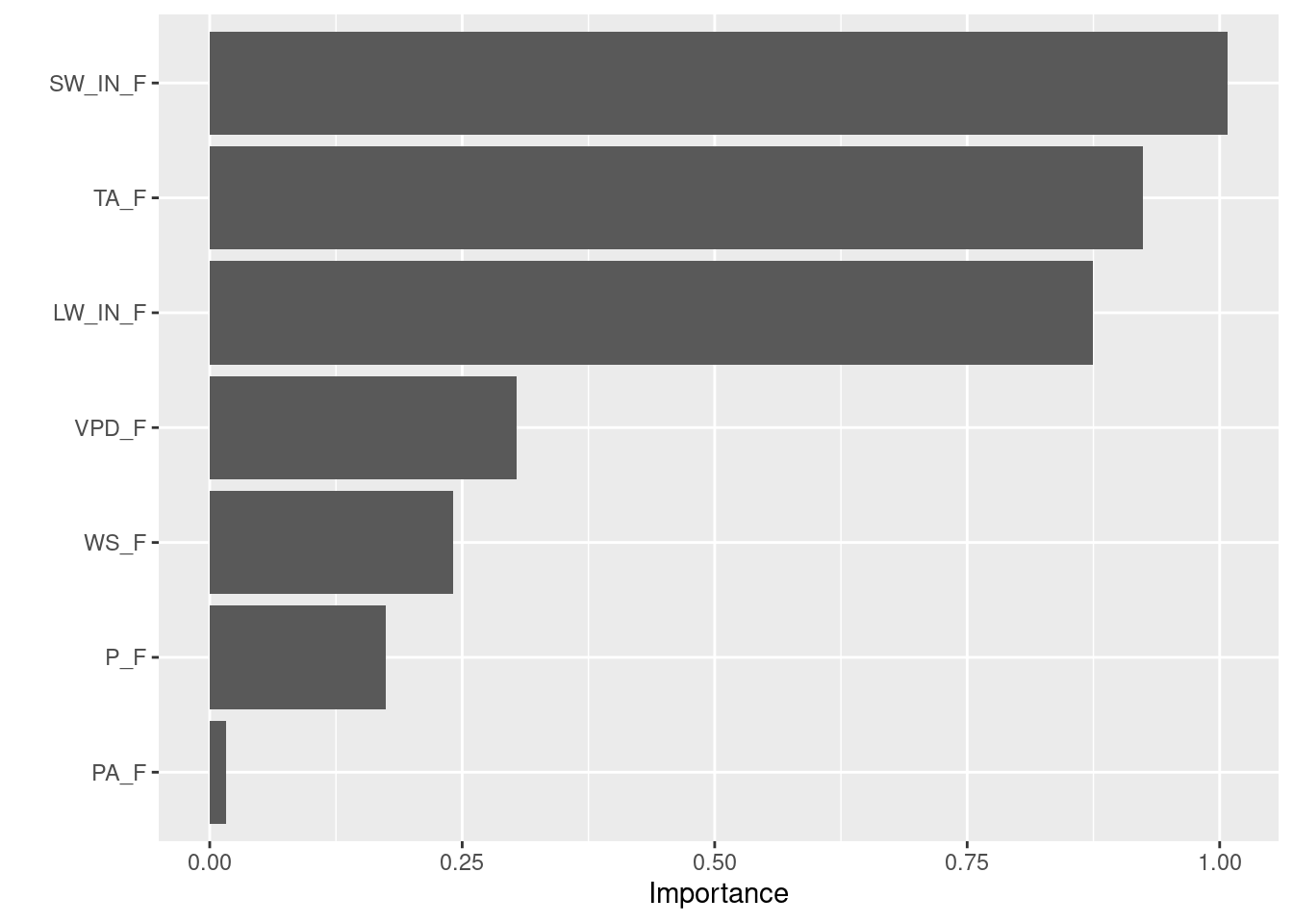
This indicates that shortwave radiation (‘SW_IN_F’) is the most important variable for modelling GPP here. I.e., the model performance degrades most (the RMSE increases most) if the information in shortwave radiation is lost. On the other extreme, atmospheric pressure adds practically no information to the model. This variable may therefore well be dropped from the model.

12.2 Partial dependence plots

We may not only want to know how important a certain variable is for modelling, but also how it influences the predictions. Is the relationship positive or negative? Is the sensitivity of predictions equal across the full range of the predictor? Again, model-agnostic approaches exist for determining the functional relationships (or partial dependencies) for predictors in a model. Partial dependence plots (PDP) give insight on the marginal effect of a single predictor variable on the response - all else equal. The algorithm to create PDPs goes as follows (adapted from Boehmke & Greenwell (2019)):

For a selected predictor (x)
1. Construct a grid of N evenly spaced values across the range of x: {x1, x2, ..., xN}
2. For i in {1,...,N} do
     | Copy the training data and replace the original values of x with the constant xi
     | Apply the fitted ML model to obtain vector of predictions for each data point.
     | Average predictions across all data points.
   End
3. Plot the averaged predictions against x1, x2, ..., xj

Figure 12.1: Visualisation of Partial Dependence Plot algorithm from Boehmke & Greenwell (2019). Here, Gr_Liv_Area is the variable of interest \(x\).

This algorithm is implemented by the {pdp} package:

# The predictor variables are saved in our model's recipe
preds <- 
  rf_mod$recipe$var_info |> 
  dplyr::filter(role == "predictor") |> 
  dplyr::pull(variable)

# The partial() function can take n=3 predictors at max and will try to create
# a n-dimensional visulaisation to show interactive effects. However, 
# this is computational intensive, so we only look at the simple 
# response-predictor plots
all_plots <- purrr::map(
  preds,
  ~pdp::partial(
      rf_mod,       # Model to use
      .,            # Predictor to assess
      plot = TRUE,  # Whether output should be a plot or dataframe
      plot.engine = "ggplot2"  # to return ggplot objects
    )
)

pdps <- cowplot::plot_grid(all_plots[[1]], all_plots[[2]], all_plots[[3]], 
                           all_plots[[4]], all_plots[[5]], all_plots[[6]])

pdps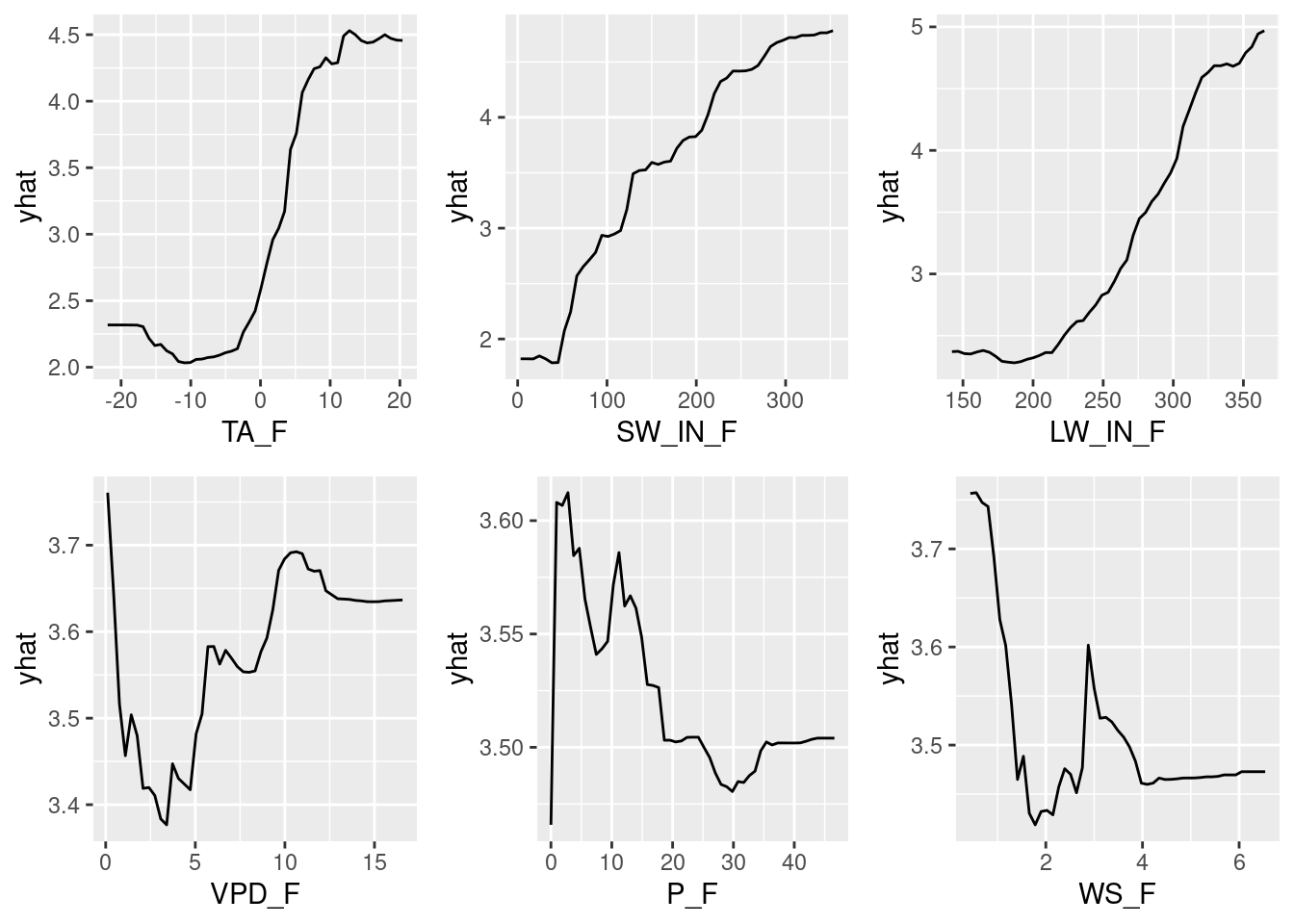

These PDPs show that the variables TA_F, SW_IN_F, and LW_IN_F have a strong effect, while VPD_F, P_F, and WS_F have a relatively small marginal effect as indicated by the small range in yhat - in line with the variable importance analysis shown above. In addition to the variable importance analysis, here we also see the direction of the effect and that how the sensitivity varies across the range of the respective predictor. For example, GPP is positively influenced by temperature (TA_F), but the effect really only starts to be expressed for temperatures above about -5\(^\circ\)C, and the positive effect disappears above about 10\(^\circ\)C. The pattern is relatively similar for LW_IN_F, which is sensible because long-wave radiation is highly correlated with temperature. For the short-wave radiation SW_IN_F, we see the saturating effect of light on GPP that we saw in previous chapters.