Sensitivity analysis and calibration interpretation

Parameter calibration can have a big impact on our modeling effort and use big computational resources. Hence, it is worth our time to explore which parameters should actually be calibrated (the ones that impact the simulations greatly) and to examine if the calibration routines behave as expected. This vignette explains how to perform a simple parameter sensitivity analysis for the P-model and how to interpret the outputs of the calibration using the BayesianTools package.

Morris sensitivity analysis

The Morris method for global sensitivity analysis allows to explore which parameters have the biggest influence on the model fit. In this example, we will quantify how different values of the calibratable model parameters lead to more variability in the match between GPP predicted by the P-model and GPP observations. It would be wise to repeat this exercise for various targets because they may be simulated by equations in the P-model that involve different model parameters.

If the P-model has very low sensitivity to a certain parameter, calibrating it will not improve the model substantially. But if it’s very sensitive to another parameter, calibrating this second parameter could improve the P-model fit greatly. We should spend our computational resources on calibrating the parameters to which the model is most sensitive.

First of all, let’s define a function which measures the agreement between GPP predictions from the P-model and GPP observations, for a set of values of the calibratable parameters. It computes the normal log-likelihood of the GPP predictions, given the observed GPP and its uncertainty. We want to see how sensitive this function is to changes in the parameter values.

# Define log-likelihood function
ll_pmodel <- function(
    par_v                 # a vector of all calibratable parameters including errors
){
  rsofun::cost_likelihood_pmodel(        # reuse likelihood cost function
    par_v,
    obs = rsofun::p_model_validation,
    drivers = rsofun::p_model_drivers,
    targets = "gpp"
  )
}

# Compute log-likelihood for a given set of parameters
ll_pmodel( par_v = c(
  kphio              = 0.09423773, # setup ORG in Stocker et al. 2020 GMD
  kphio_par_a        = 0.0,        # set to zero to disable temperature-dependence of kphio
  kphio_par_b        = 1.0,
  soilm_thetastar    = 0.6 * 240,  # to recover old setup with soil moisture stress
  soilm_betao        = 0.0,
  beta_unitcostratio = 146.0,
  rd_to_vcmax        = 0.014,      # value from Atkin et al. 2015 for C3 herbaceous
  tau_acclim         = 30.0,
  kc_jmax            = 0.41,
  error_gpp          = 0.9         # value from previous simulations
))
#> [1] -45306.56

Some parameters are constrained by their physical interpretation (e.g. kphio > 0) and it’s also necessary to provide a bounded parameter space for Morris’ method to sample the parameter space. We define the parameter space by their lower and upper bounds.

# best parameter values (from previous literature)
par_cal_best <- c(
    kphio              = 0.09423773,
    kphio_par_a        = -0.0025,
    kphio_par_b        = 20,
    soilm_thetastar    = 0.6*240,
    soilm_betao        = 0.2,
    beta_unitcostratio = 146.0,
    rd_to_vcmax        = 0.014,
    tau_acclim         = 30.0,
    kc_jmax            = 0.41,
    error_gpp          = 1
  )

# lower bound
par_cal_min <- c(
    kphio              = 0.03,
    kphio_par_a        = -0.004,
    kphio_par_b        = 10,
    soilm_thetastar    = 0,
    soilm_betao        = 0,
    beta_unitcostratio = 50.0,
    rd_to_vcmax        = 0.01,
    tau_acclim         = 7.0,
    kc_jmax            = 0.2,
    error_gpp          = 0.01
  )

# upper bound
par_cal_max <- c(
    kphio              = 0.15,
    kphio_par_a        = -0.001,
    kphio_par_b        = 30,
    soilm_thetastar    = 240,
    soilm_betao        = 1,
    beta_unitcostratio = 200.0,
    rd_to_vcmax        = 0.1,
    tau_acclim         = 60.0,
    kc_jmax            = 0.8,
    error_gpp          = 4
  )

We use the morris() function from the {sensitivity} package to perform the sensitivity analysis. As a target function, we will use the posterior density (log-likelihood) of the parameters given the GPP data which we obtain via the function BayesianTools::createBayesianSetup(). Note that, because of using a uniform prior, the posterior distribution is proportional to the GPP log-likelihood (defined previously) wherever the parameter values are feasible and zero outside of the parameter ranges.

morris_setup <- BayesianTools::createBayesianSetup(
  likelihood = ll_pmodel,
  prior = BayesianTools::createUniformPrior(par_cal_min, par_cal_max, par_cal_best),
  names = names(par_cal_best)
)

In the following chunk, we run the Morris sensitivity analysis, using a grid with r=1000 values for each parameter and a one-at-a-time design. Running the sensitivity analysis may take a few minutes, even for this small example dataset, and is still computationally cheaper than running the parameter calibration.

set.seed(432)
morrisOut <- sensitivity::morris(
  model = morris_setup$posterior$density,
  factors = names(par_cal_best), 
  r = 1000, 
  design = list(type = "oat", levels = 20, grid.jump = 3), 
  binf = par_cal_min, 
  bsup = par_cal_max, 
  scale = TRUE)

The analysis evaluates the variability of the target function, i.e. the log-likelihood, for several points across the parameter space. It is an approximation of the derivatives of the log-likelihood with respect to the model parameters. Statistics \(\mu *\) and \(\sigma\) can be interpreted as the mean absolute derivative and the standard deviation of the derivative, respectively. The higher the value of these statistics for a given parameter, the more influential the parameter is.

# Summarise the morris output
morrisOut.df <- data.frame(
  parameter = names(par_cal_best),
  mu.star = apply(abs(morrisOut$ee), 2, mean, na.rm = T),
  sigma = apply(morrisOut$ee, 2, sd, na.rm = T)
) %>%
  arrange( mu.star )

morrisOut.df |>
  tidyr::pivot_longer( -parameter, names_to = "variable", values_to = "value") |>
  ggplot(aes(
    reorder(parameter, value),
    value, 
    fill = variable),
    color = NA) +
  geom_bar(position = position_dodge(), stat = 'identity') +
  scale_fill_brewer("", labels = c('mu.star' = expression(mu * "*"),
                                   'sigma' = expression(sigma)),
                    palette = "Greys") +
  theme_classic() +
  theme(
    axis.text = element_text(size = 6),
    axis.title = element_blank(),
    legend.position = c(0.05, 0.95), legend.justification = c(0.05, 0.95)
  )
#> Warning: A numeric `legend.position` argument in `theme()` was deprecated in ggplot2
#> 3.5.0.
#> ℹ Please use the `legend.position.inside` argument of `theme()` instead.
#> This warning is displayed once every 8 hours.
#> Call `lifecycle::last_lifecycle_warnings()` to see where this warning was
#> generated.

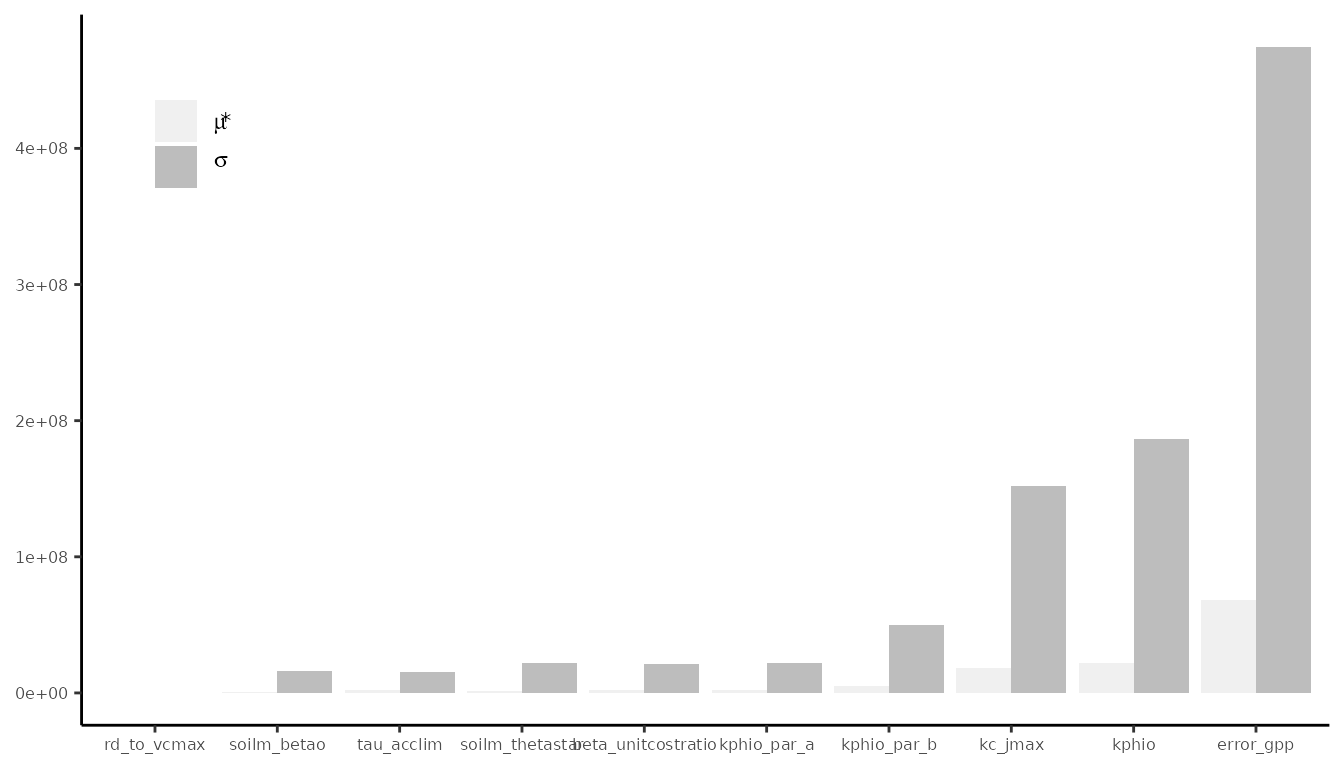
The outcome of the Morris sensitivity analysis depends strongly on the choice of parameter ranges and how parameters interact with each other in the underlying model. In this example, we constrained the parameters based on their physical meaning (e.g. soilm_betao should be in [0,1]) and the site FR-Pue where the data is coming from (e.g. kphio_par_b around 25\(^{o}\)C). When observing the figure above, we notice that parameters kphio and kc_jmax have a high impact on the model fit (big \(\mu *\)), but also the magnitude of this dependence of GPP on the two parameters changes across the parameter space (big \(\sigma\)). This happens because parameters interact in the light use efficiency calculation and the calibration may be harder and require data from several sites.

The log-likelihood is most sensitive to err_gpp with a very large variation in the magnitude of this dependence. This makes sense because for higher values of the standard deviation the normal likelihood is flatter (and similar log-likelihood values are calculated, whether the model predictions using the rest of parameters are good or bad) and for lower err_gpp values the likelihood is pointy (hence good model fits achieve a big log-likelihood value and and poor model fits, a very small value).

To help you interpret this sensitivity analysis and better understand the parameter-model relationship, it may be wise to run it several times for different parameter ranges and validation data. Note how rd_to_vcmax does not affect GPP, but it would actually affect dark respiration predictions, so trait data could also be added for validation.

Interpretation of Bayesian calibration routine

It is always important to check the convergence of the MCMC algorithm used for the Bayesian calibration. Here we show some plots and statistics that may help you assess whether the parameter calibration has converged.

According to the previous sensitivity analysis, calibrating the error parameter for GPP and the quantum yield efficiency parameters will have a high impact on the model fit. Let’s run the calibration:

set.seed(2023)

# Define calibration settings
settings_calib <- list(
  method = "BayesianTools",
  metric = rsofun::cost_likelihood_pmodel,
  control = list(
    sampler = "DEzs",
    settings = list(
      burnin = 3000,
      iterations = 9000,
      nrChains = 3,        # number of independent chains
      startValue = 3       # number of internal chains to be sampled
    )),
  par = list(
    kphio = list(lower = 0.03, upper = 0.15, init = 0.05),
    kphio_par_a = list(lower = -0.004, upper = -0.001, init = -0.0025),
    kphio_par_b = list(lower = 10, upper = 30, init =25),
    err_gpp = list(lower = 0.1, upper = 3, init = 0.8)
  )
)

# Calibrate kphio-related parameters and err_gpp 
par_calib <- calib_sofun(
  drivers = p_model_drivers,
  obs = p_model_validation,
  settings = settings_calib,
  par_fixed = list(
    soilm_thetastar    = 0.6*240,
    soilm_betao        = 0.2,
    beta_unitcostratio = 146.0,
    rd_to_vcmax        = 0.014,
    tau_acclim         = 30.0,
    kc_jmax            = 0.41),
  targets = "gpp"
)

# This code takes 15 minutes to run

BayesianTools makes it easy to produce the trace plot of the MCMC chains and the posterior density plot for the parameters. Trace plots show the time series of the sampled chains, which should reach a stationary state. One can also choose a burnin visually, to discard the early iterations and keep only the samples from the stationary distribution to which they converge. We set above from previous runs, and those iterations are not shown by the following trace plot. The samples after the burnin period should be used for inference.

plot(par_calib$mod)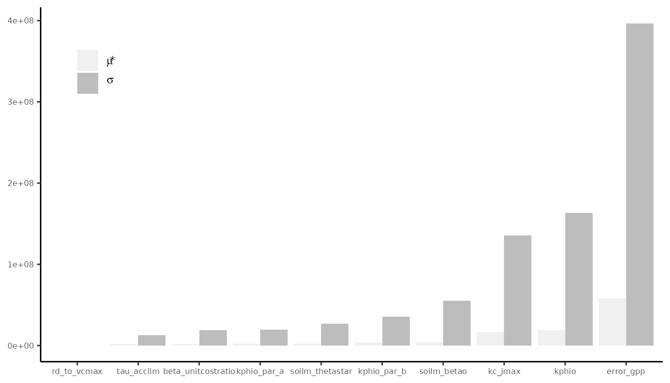

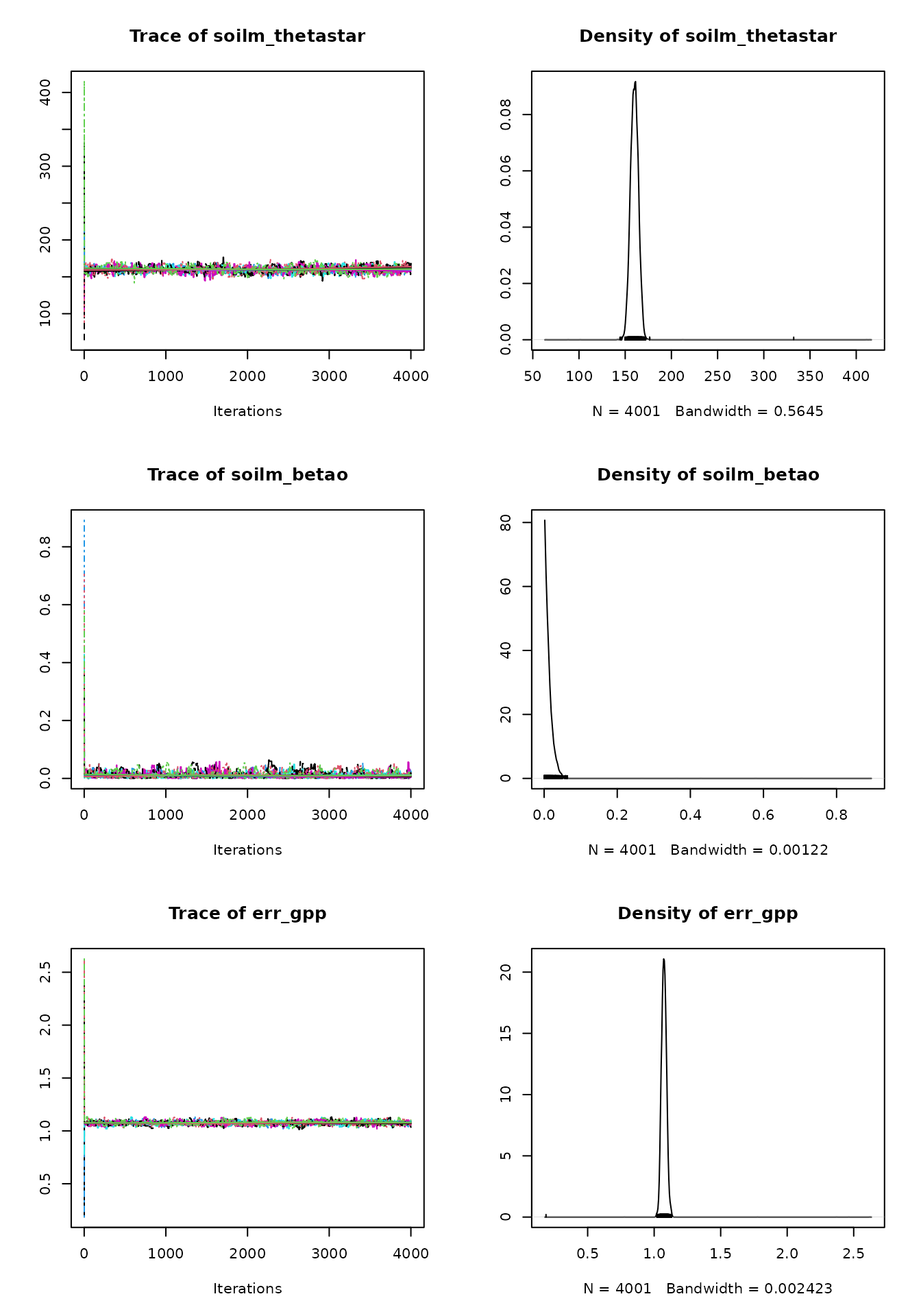
The posterior density plots may be lumpy. In this case it’s advisable to run the MCMC algorithm for more iterations, in order to get a better estimate of the parameters’ posterior distributions. A good posterior should look more gaussian (although it can be skewed). A multimodal density indicates that the MCMC is still exploring the parameter space and hasn’t converged yet. The posteriors can be plotted against the priors using BayesianTools::marginalPlot().

When convergence has been reached, the oscillation of the time series should look like white noise. It’s normal that consecutive MCMC samples are correlated because of the sampling algorithm’s nature, but the presence of a more general trend indicates that convergence hasn’t been reached.

Looking at the correlation between chains for different parameters is also helpful because parameter correlation may slow down convergence, or the chains may oscillate in the multivariate posterior space. In this calibration we expect parameter samples to be somewhat correlated, especially kphio_par_a and kphio_par_b because they specify the shape of the temperature dependence of the quantum yield efficiency, \(\varphi_o(T)\). We can also see that err_gpp is correlated with kphio (to which the P-model is very sensitive), since the error represents how good the model fits the observed GPP.

correlationPlot(par_calib$mod, thin = 1)   # use all samples, no thinning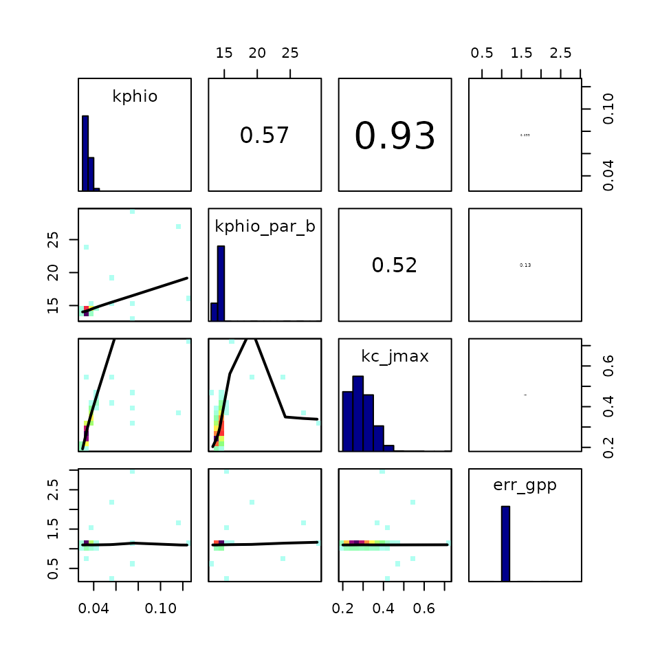

In addition to visualizations, it’s helpful to compute some convergence diagnostics, like the Gelman-Brooks-Rubin (GBR) potential scale factors. This diagnostic compares the variance within chains to that across chains and should progressively get closer to 1. It is common in the literature (Gelman, A., Carlin, J.B., Stern, H.S., Rubin, D.B.: Bayesian Data Analysis, 2nd edn. Chapman & Hall, London (2004)) to accept convergence with a GBR between 1.05 and 1.1.

gelmanDiagnostics(par_calib$mod)
#> Potential scale reduction factors:
#> 
#>             Point est. Upper C.I.
#> kphio             1.00       1.01
#> kphio_par_a       1.01       1.01
#> kphio_par_b       1.01       1.02
#> err_gpp           1.02       1.05
#> 
#> Multivariate psrf
#> 
#> 1.03

Finally, the parameter MAP estimates can be derived from the chains (that converged) after removing the burnin period. They can be seen, next to other statistics, using the summary function from the BayesianTools library.

summary(par_calib$mod)
#> # # # # # # # # # # # # # # # # # # # # # # # # # 
#> ## MCMC chain summary ## 
#> # # # # # # # # # # # # # # # # # # # # # # # # # 
#>  
#> # MCMC sampler:  DEzs 
#> # Nr. Chains:  9 
#> # Iterations per chain:  2001 
#> # Rejection rate:  0.802 
#> # Effective sample size:  2181 
#> # Runtime:  942.881  sec. 
#>  
#> # Parameters
#>               psf    MAP   2.5% median  97.5%
#> kphio       1.004  0.046  0.045  0.046  0.047
#> kphio_par_a 1.005 -0.002 -0.002 -0.002 -0.002
#> kphio_par_b 1.008 17.256 16.638 17.262 17.957
#> err_gpp     1.022  1.175  1.140  1.174  1.214
#> 
#> ## DIC:  5022.956 
#> ## Convergence 
#>  Gelman Rubin multivariate psrf:  1.035 
#>  
#> ## Correlations 
#>              kphio kphio_par_a kphio_par_b err_gpp
#> kphio        1.000      -0.294       0.027   0.142
#> kphio_par_a -0.294       1.000       0.285   0.013
#> kphio_par_b  0.027       0.285       1.000   0.022
#> err_gpp      0.142       0.013       0.022   1.000

More details on diagnosing MCMC convergence can be found in this vignette from BayesianTools and this blogpost.

Plotting P-model output after calibration

After we have run and checked the calibration, let’s see how the model performs.

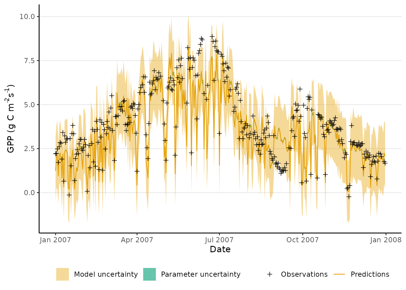
To compute the credible intervals for GPP prediction, we ran the P-model for 600 samples from the posterior distribution of the calibrated parameters. As a result, we obtain the posterior distribution of modeled GPP at each time step and also the posterior distribution of predicted GPP, which incorporates the Gaussian model error.

# Evaluation of the uncertainty coming from the model parameters' uncertainty

# Sample parameter values from the posterior distribution
samples_par <- getSample(par_calib$mod, 
                             thin = 30,              # get every 30th sample
                             whichParameters = 1:4) |>  
  as.data.frame() |>
  dplyr::mutate(mcmc_id = 1:n()) |>
  tidyr::nest(.by = mcmc_id, .key = "pars")

run_pmodel <- function(sample_par){
  # Function that runs the P-model for a sample of parameters
  # and also adds the new observation error
  
  out <- runread_pmodel_f(
    drivers = p_model_drivers,
    par =  list(                      # copied from par_fixed above
      kphio = sample_par$kphio,
      kphio_par_a = sample_par$kphio_par_a,
      kphio_par_b = sample_par$kphio_par_b,
      soilm_thetastar    = 0.6*240,
      soilm_betao        = 0.2,
      beta_unitcostratio = 146.0,
      rd_to_vcmax        = 0.014,
      tau_acclim         = 30.0,
      kc_jmax            = 0.41)       # value from posterior
  )
  
  # return modelled GPP and prediction for a new GPP observation
  gpp <- out$data[[1]][, "gpp"]
  data.frame(gpp = gpp, 
             gpp_pred = gpp + rnorm(n = length(gpp), mean = 0, 
                                   sd = sample_par$err_gpp),
             date = out$data[[1]][, "date"])
}

set.seed(2023)
# Run the P-model for each set of parameters
pmodel_runs <- samples_par |>
  dplyr::mutate(sim = purrr::map(pars, ~run_pmodel(.x))) |>
  # format to obtain 90% credible intervals
  dplyr::select(mcmc_id, sim) |>
  tidyr::unnest(sim) |>
  dplyr::group_by(date) |>
  # compute quantiles for each day
  dplyr::summarise(
    gpp_q05 = quantile(gpp, 0.05, na.rm = TRUE),
    gpp = quantile(gpp, 0.5, na.rm = TRUE),          # get median
    gpp_q95 = quantile(gpp, 0.95, na.rm = TRUE),
    gpp_pred_q05 = quantile(gpp_pred, 0.05, na.rm = TRUE),
    gpp_pred_q95 = quantile(gpp_pred, 0.95, na.rm = TRUE)
  )

Below we plot the first year of observed GPP (in black) against the predicted GPP (in grey), computed as the median of the posterior distribution of modeled GPP. This information is accompanied by the 90% credible interval for predicted GPP (shaded in blue, very narrow) and the 90% predictive interval (shaded in grey). We can see that the parameter uncertainty captured in the credible interval is quite small, in comparison to the model uncertainty captured by the predictive interval.

# Plot the credible intervals computed above
# for the first year only
plot_gpp_error <- ggplot(data = pmodel_runs |>
    dplyr::slice(1:365)) +             # Plot only first year
  geom_ribbon(
    aes(ymin = gpp_q05, 
        ymax = gpp_q95,
        x = date),
    fill = 'blue', alpha = 0.5) +
  geom_ribbon(
    aes(ymin = gpp_pred_q05, 
        ymax = gpp_pred_q95,
        x = date),
    fill = 'grey40', alpha = 0.2) +
  geom_line(
    aes(
      date,
      gpp
    ),
    colour = "grey40",
    alpha = 0.8
  ) +
  theme_classic() +
  theme(panel.grid.major.y = element_line()) +
  labs(
    x = 'Date',
    y = expression(paste("GPP (g C m"^-2, "s"^-1, ")"))
  )

# Define GPP validation data (first year)
validation_data <- p_model_validation$data[[1]][1:365, ]

# Include observations in the plot
plot_gpp_error +  
  geom_line(
    data = validation_data,
    aes(
      date,
      gpp
    ),
    alpha = 0.8
  )

Josefa Arán

Morris sensitivity analysis

Interpretation of Bayesian calibration routine

Plotting P-model output after calibration

About

Resources