Potential cumulative water deficit
Beni Stocker
2026-03-08
Source:vignettes/potential_cwd.Rmd
potential_cwd.Rmd
library(readr)
library(dplyr)
library(tidyr)
library(here)
library(lubridate)
library(patchwork)
library(extRemes)
library(ggplot2)
library(cwd)
library(visdat)
library(recipes)
# library(readxl)
# library(zoo)
# library(ggpubr)
A potential cumulative water deficit can be calculated using net radiation and the potential evapotranspiration (PET). Here, we calculate PET based on net radiation and the approach by Priestley & Taylor (1972) as implemented by Davis et al. (2017). Necessary functions are part of the {cwd} package.
Prepare data
Read data from the example FLUNXET file contained in this repository.
df <- cwd:::df_FR_PUE |> # readRDS(file = paste0(here(), "/data/df_fr-pue.rds")) |>
   # convert to from kPA to Pa (SI units are used for inputs to functions in the package)
   mutate(PA_F = 1e3 * PA_F) |>
   # Convert TIMESTAMP to Date format
   mutate(TIMESTAMP = ymd(TIMESTAMP))


# df <- readRDS(file = paste0(here(), "/data/df_fr-pue.rds")) |>
#    # convert to from kPA to Pa (SI units are used for inputs to functions in the package)
#    mutate(PA_F = 1e3 * PA_F)

#visdat::vis_miss(df)
Some net radiation data is missing. Impute missing values by KNN.
pp <- recipes::recipe(
  NETRAD ~ SW_IN_F_MDS + LW_IN_F_MDS + TA_F_MDS,
  data = df |>
    drop_na(SW_IN_F_MDS, LW_IN_F_MDS, TA_F_MDS)
) |>
  recipes::step_center(
    recipes::all_numeric(),
    -recipes::all_outcomes()
  ) |>
  recipes::step_scale(
    recipes::all_numeric(),
    -recipes::all_outcomes()
  ) |>
  recipes::step_impute_knn(
    recipes::all_outcomes(),
    neighbors = 5
  )

pp_prep <- recipes::prep(
  pp,
  training = df |>
    drop_na(SW_IN_F_MDS, LW_IN_F_MDS, TA_F_MDS)
)

df_baked <- recipes::bake(
  pp_prep,
  new_data = df
)

# fill missing with gap-filled
df <- df |>
  dplyr::bind_cols(
    df_baked |>
      dplyr::select(
        NETRAD_filled = NETRAD)
  ) |>
  dplyr::mutate(
    NETRAD = ifelse(is.na(NETRAD), NETRAD_filled, NETRAD)
    #qc = ifelse(is.na(netrad), TRUE, FALSE)
  ) |>
  dplyr::select(
    -NETRAD_filled
  )

#visdat::vis_miss(df)Visualise, contrasting to observed ET after conversion of energy to mass units
Convert latent heat flux (W/m2) to evapotranspiration in mass units (mm/d).
# tested: identical results are obtained with:
# bigleaf::LE.to.ET(LE_F_MDS, TA_F_MDS)* 60 * 60 * 24
le_to_et <- function(le, tc, patm){
  1000 * 60 * 60 * 24 * le / (cwd::calc_enthalpy_vap(tc) * cwd::calc_density_h2o(tc, patm))
}

df <- df |>
  mutate(et = le_to_et(LE_F_MDS, TA_F_MDS, PA_F))
Plot mean seasonal cycle.
# df |>
#   mutate(TIMESTAMP = lubridate::as_date(as_datetime(TIMESTAMP_END)))

df |>
  mutate(doy = lubridate::yday(TIMESTAMP)) |>
  group_by(doy) |>
  summarise(
    et = mean(et),
    pet = mean(pet)
  ) |>
  ggplot() +
  geom_line(aes(doy, et, color = "ET")) +
  geom_line(aes(doy, pet, color = "PET")) +
  labs(
    x = "Day of year",
    y = expression(paste("Water vapour mass flux (mm d"^-1, ")"))
  ) +
  theme_classic()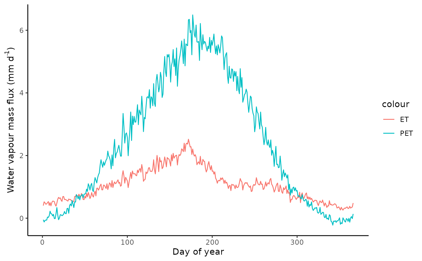
Cumulating PET - P
Check annual totals.
adf <- df |>
  mutate(year = year(TIMESTAMP)) |>
  group_by(year) |>
  summarise(pet = sum(pet), prec = sum(P_F))

adf |>
  tidyr::pivot_longer(cols = c(pet, prec), names_to = "Flux") |>
  ggplot(aes(x = year, y = value, color = Flux)) +
  geom_line() +
  labs(y = "Flux (mm/yr)") +
  theme_classic()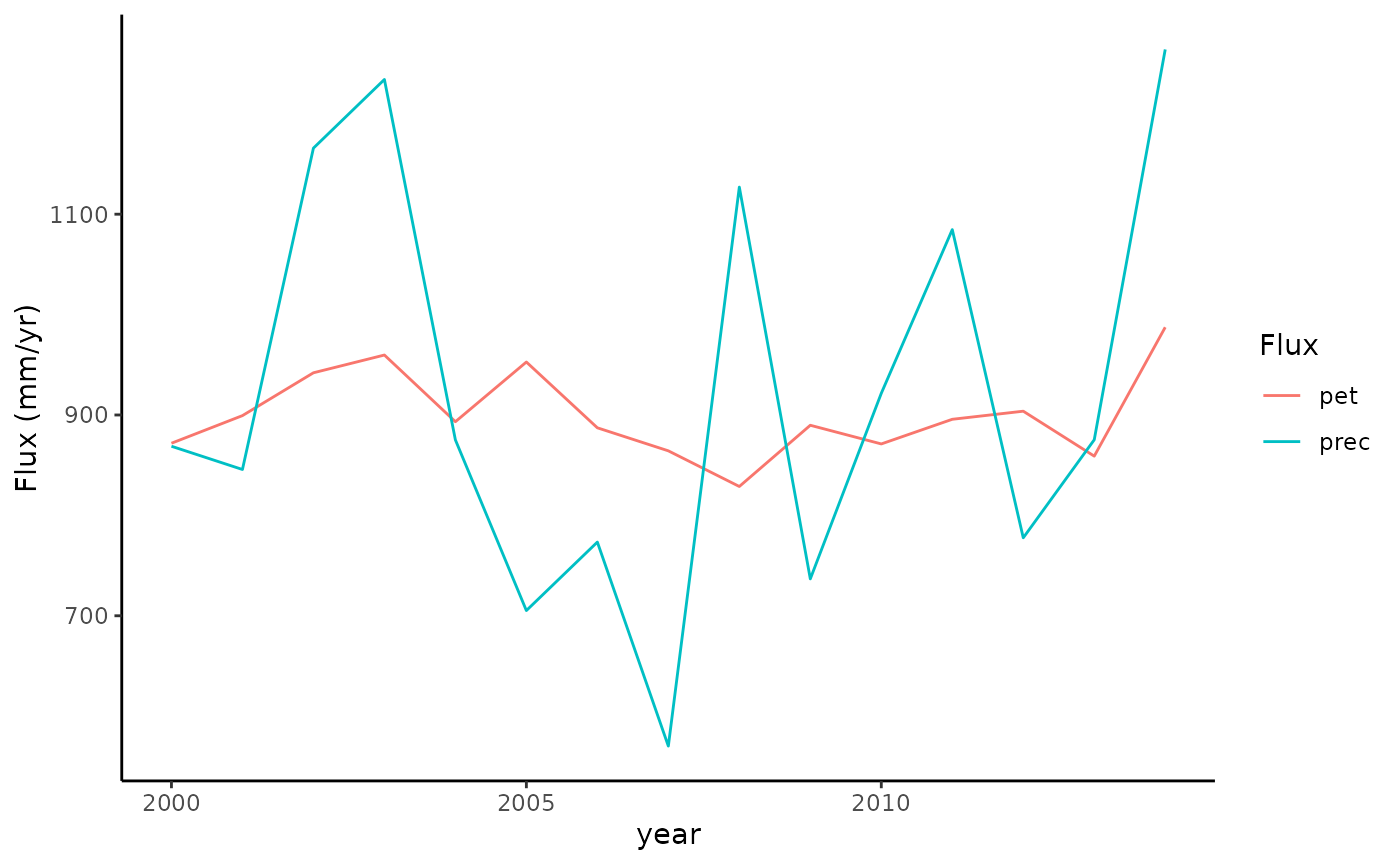
In some cases, the mean annual PET may be larger than the mean annual precipitation (P), leading to a steady long-term increase of a potential cumulative water deficit. This is the case here (see plot above).
df |>
  mutate(pcwd = cumsum(pet - P_F)) |>
  ggplot(aes(TIMESTAMP, pcwd)) +
  geom_line() +
  theme_classic()
This indicates a need to re-set the potential cumulative water deficit calculation. Let’s determine the wettest month from the available years of data and reset the cumulative water deficit each year in that month. The plot below shows the average P - PET for each month. November is the wettest month at this site.
mdf_mean <- df |>
  mutate(month = lubridate::month(TIMESTAMP),
         pwbal = P_F - pet) |>
  group_by(month) |>
  summarise(
    pwbal = sum(pwbal)
  )

mdf_mean |>
  ggplot(aes(as.factor(month), pwbal)) +
  geom_bar(stat = "identity") +
  theme_classic()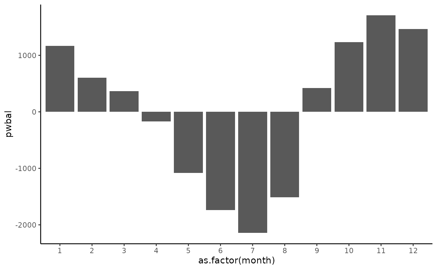
Therefore, we re-set the accumulation of the water deficit each year on the first day after November (in other words, 1st of December)
# determine the day-of-year of the first day of the month after the wettest month
doy_reset <- lubridate::yday(lubridate::ymd("2000-11-01") + lubridate::dmonths(1))
Distribution of daily precipitation and PET to aid choosing an
absolute threshold (threshold_terminate_absolute)
determining the end of a CWD event (see next).
df |>
  ggplot(aes(P_F, after_stat(density))) +
  geom_density(bw = 1) +
  xlim(-1, 30)
## Warning: Removed 110 rows containing non-finite outside the scale range
## (`stat_density()`).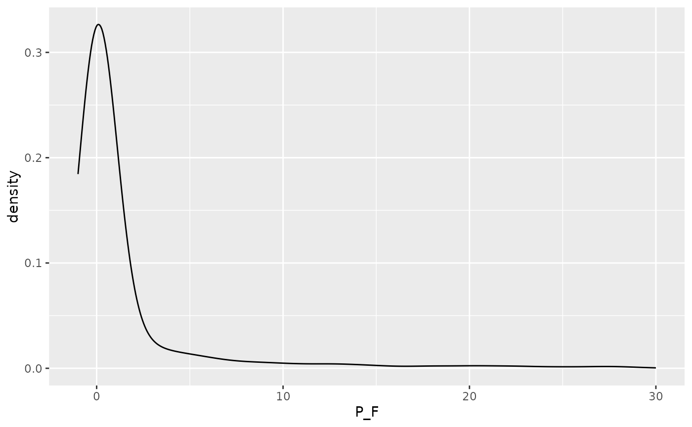
df |>
  ggplot(aes(pet, after_stat(density))) +
  geom_density(bw = 1) +
  xlim(-1, 30)
## Warning: Removed 7 rows containing non-finite outside the scale range
## (`stat_density()`).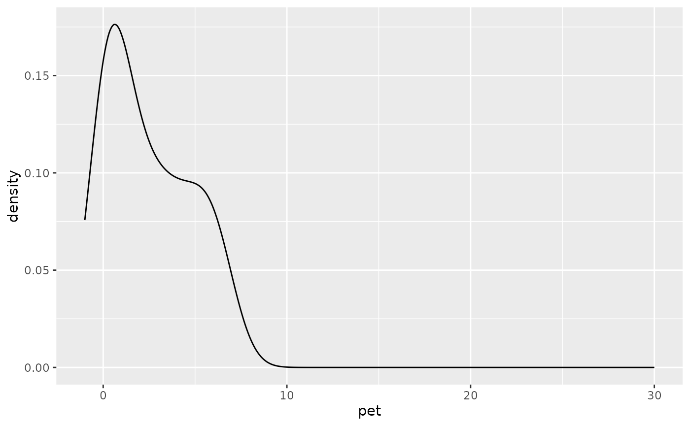
Get the potential cumulative water deficit time series and individual
events. Note that we use the argument doy_reset
here to force a re-setting of the potential cumulative water deficit on
that same day each year. A relative and an absolute option are possible
for determining the threshold to which a CWD has to be reduced to to
terminate the event: 1) threshold_terminate: Set the
threshold relative to maximum CWD attained. Defaults to 0, meaning that
the CWD has to be fully compensated by water infiltration into the soil
to terminate a CWD event. 2) threshold_terminate_absolute:
threshold determining end of event as thresh_terminate but
in absolute terms (in mm d-1). Default set to NA. If no
option is given, the function defaults to the relative threshold.
Option 1: CWD calculation using a relative threshold:
df <- df |>
  mutate(pwbal = P_F - pet)

out_cwd <- cwd(
  df,
  varname_wbal = "pwbal",
  varname_date = "TIMESTAMP",
  thresh_terminate = 0,
  thresh_drop = 0.0,
  doy_reset = doy_reset
  )
Retain only events of a minimum length of 20 days.
out_cwd$inst <- out_cwd$inst |>
  filter(len >= 20)
Plot the potential cumulative water deficit time series and events.
ggplot() +
  geom_rect(
    data = out_cwd$inst,
    aes(xmin = date_start, xmax = date_end, ymin = 0, ymax = max( out_cwd$df$deficit)),
    fill = rgb(0,0,0,0.3),
    color = NA) +
  geom_line(data  =  out_cwd$df, aes(TIMESTAMP, deficit), color = "tomato") +
  theme_classic() +
  ylim(0, max(out_cwd$df$deficit)) +
  labs(
    x = "Date",
    y = "Potential cumulative water deficit (mm)"
    )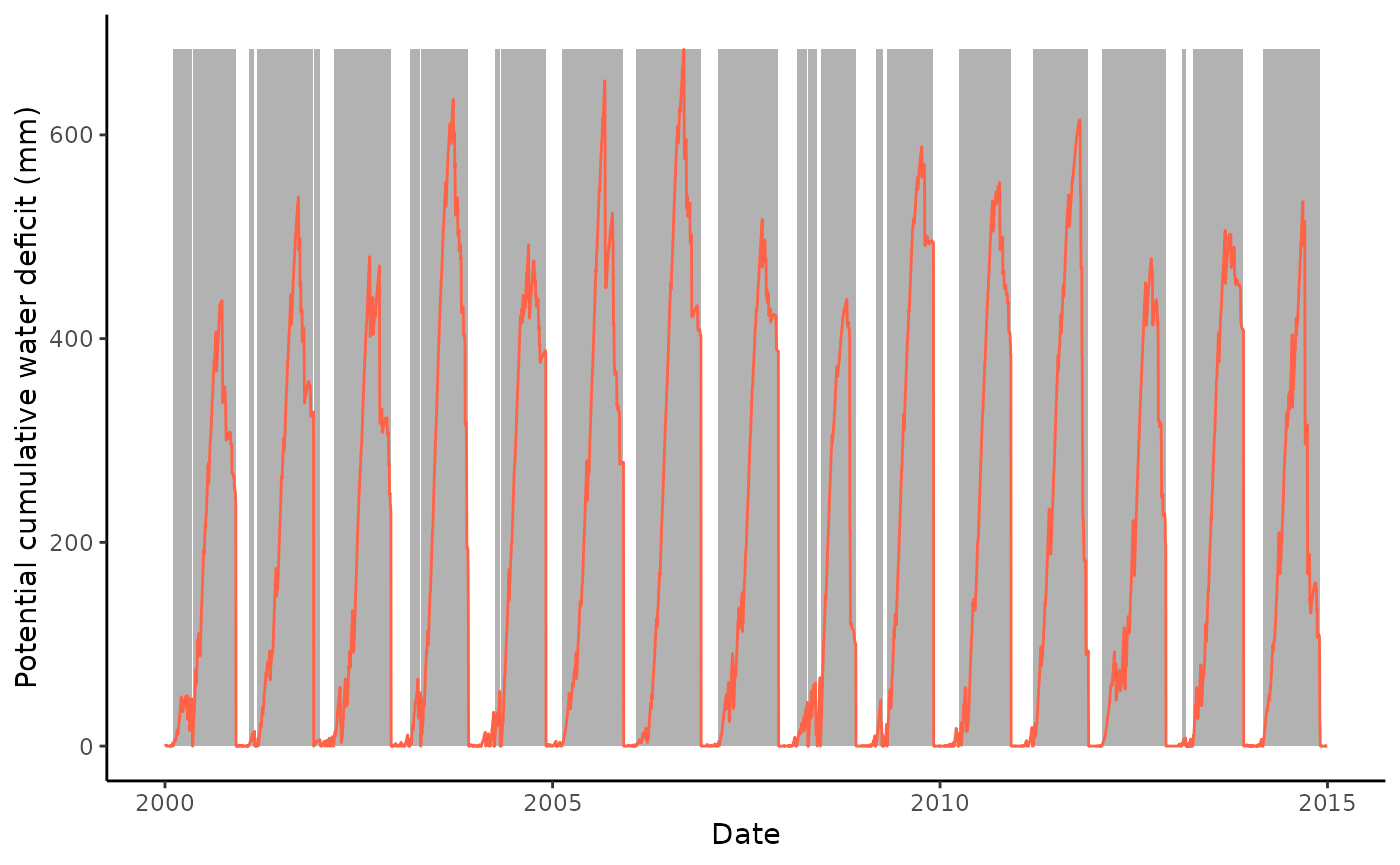
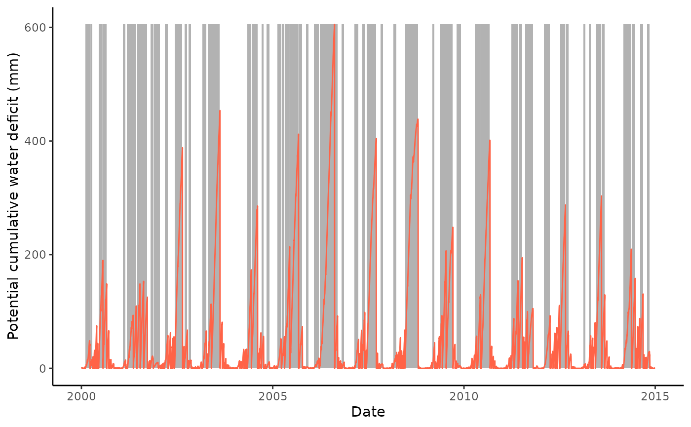
Option 2: CWD calculation using an absolute threshold, here 10mm. The deficit reset is not prescribed through a given DOY here but resets once the deficit falls below the threshold. Absolute thresholds should be selected based on the regional water balance.
df <- df |>
  mutate(pwbal = P_F - pet)

out_cwd <- cwd(
  df,
  varname_wbal = "pwbal",
  varname_date = "TIMESTAMP",
  thresh_terminate_absolute = 10,
  thresh_drop = 0.0
  )
Retain only events of a minimum length of 20 days.
out_cwd$inst <- out_cwd$inst |>
  filter(len >= 20)
Plot the potential cumulative water deficit time series and events.
ggplot() +
  geom_rect(
    data = out_cwd$inst,
    aes(xmin = date_start, xmax = date_end, ymin = 0, ymax = max( out_cwd$df$deficit)),
    fill = rgb(0,0,0,0.3),
    color = NA) +
  geom_line(data  =  out_cwd$df, aes(TIMESTAMP, deficit), color = "tomato") +
  theme_classic() +
  ylim(0, max(out_cwd$df$deficit)) +
  labs(
    x = "Date",
    y = "Potential cumulative water deficit (mm)"
    )
References
Davis, T. W., Prentice, I. C., Stocker, B. D., Thomas, R. T., Whitley, R. J., Wang, H., Evans, B. J., Gallego-Sala, A. V., Sykes, M. T., & Cramer, W. (2017). Simple process-led algorithms for simulating habitats (SPLASH v.1.0): Robust indices of radiation, evapotranspiration and plant-available moisture. Geoscientific Model Development, 10(2), 689–708. https://doi.org/10.5194/gmd-10-689-2017
Priestley, C. H. B., & Taylor, R. J. (1972). On the Assessment of Surface Heat Flux and Evaporation Using Large-Scale Parameters. Monthly Weather Review, 100(2), 81–92. https://doi.org/10.1175/1520-0493(1972)100<0081:OTAOSH>2.3.CO;2