Cumulative water deficit example
Beni Stocker
2026-03-08
Source:vignettes/cwd_example.Rmd
cwd_example.Rmd
library(readr)
library(dplyr)
library(here)
library(lubridate)
library(patchwork)
library(extRemes)
library(ggplot2)
library(cwd)
This demonstrates the workflow for determining cumulative water deficit (CWD) time series and fitting an extreme value distribution to annual maxima of the CWD time series.
Prepare data
Read data from the file contained in this repository.
df <- cwd:::df_CH_LAE |>
  # convert to from kPA to Pa (SI units are used for inputs to functions in the package)
  mutate(PA_F = 1e3 * PA_F)
Convert ET to mass units
Convert latent heat flux (W/m2) to evapotranspiration in mass units (mm/d).
# tested: identical results are obtained with:
# bigleaf::LE.to.ET(LE_F_MDS, TA_F_MDS)* 60 * 60 * 24
le_to_et <- function(le, tc, patm){
  1000 * 60 * 60 * 24 * le / (cwd::calc_enthalpy_vap(tc) * cwd::calc_density_h2o(tc, patm))
}

df <- df |>
  mutate(et = le_to_et(LE_F_MDS, TA_F_MDS, PA_F))
Check annual totals.
adf <- df |>
  mutate(year = year(TIMESTAMP)) |>
  group_by(year) |>
  summarise(et = sum(et), prec = sum(P_F))

adf |>
  tidyr::pivot_longer(cols = c(et, prec), names_to = "Flux") |>
  ggplot(aes(x = year, y = value, color = Flux)) +
  geom_line() +
  labs(y = "Flux (mm/yr)")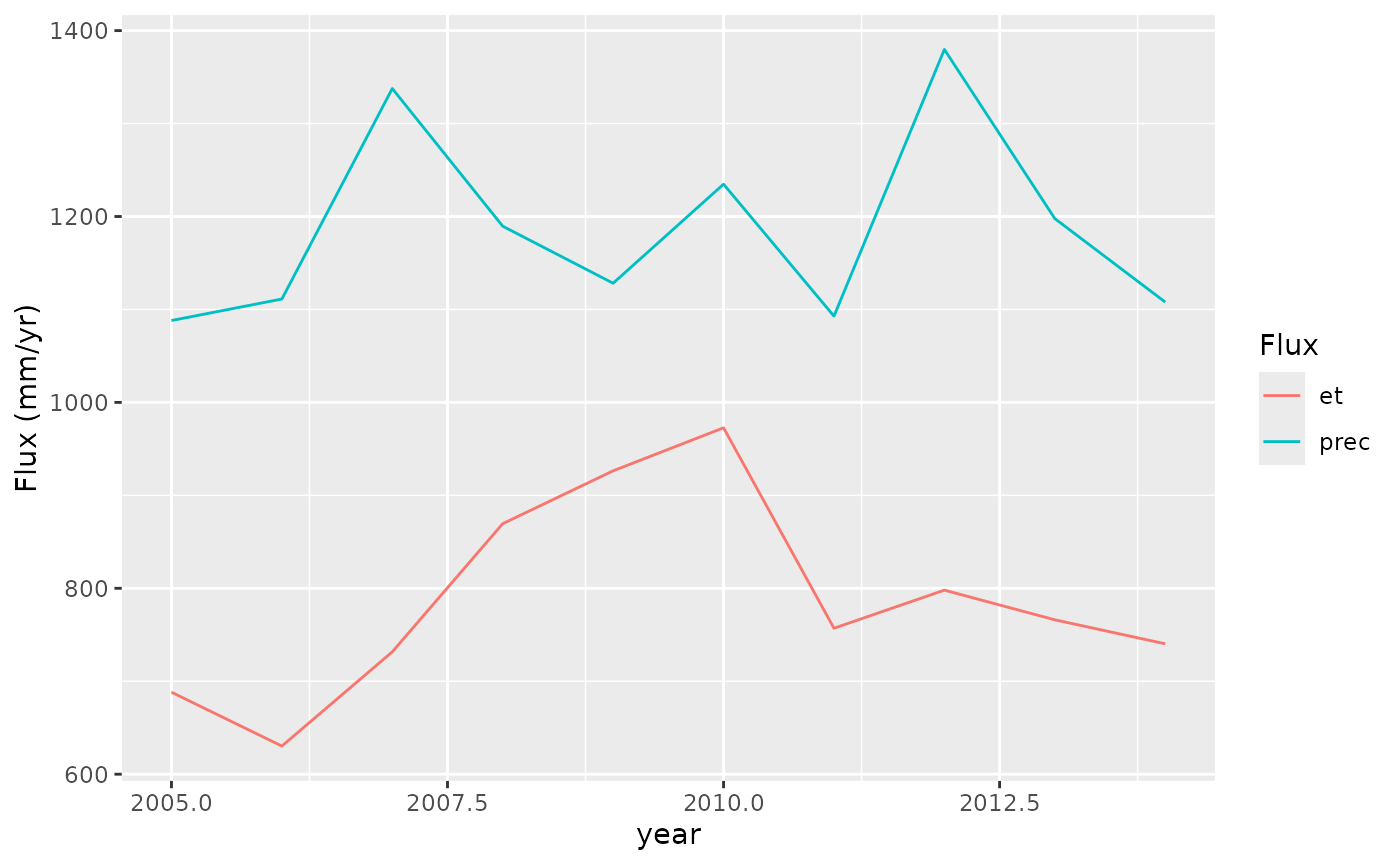
Each year, the annual precipitation is greater than ET. Hence, the water deficit will not continue accumulating over multiple years.
Simulate snow
Simulate snow accumulation and melt based on temperature and precipitation.
df <- df |>
  mutate(prec = ifelse(TA_F_MDS < 0, 0, P_F),
         snow = ifelse(TA_F_MDS < 0, P_F, 0)) |>
  cwd::simulate_snow(varnam_prec = "prec", varnam_snow = "snow", varnam_temp = "TA_F_MDS")
Visualise snow mass equivalent time series.
df |>
  ggplot(aes(TIMESTAMP, snow_pool)) +
  geom_line() +
  labs(x = "Date", y = "Snow mass equivalent (mm)")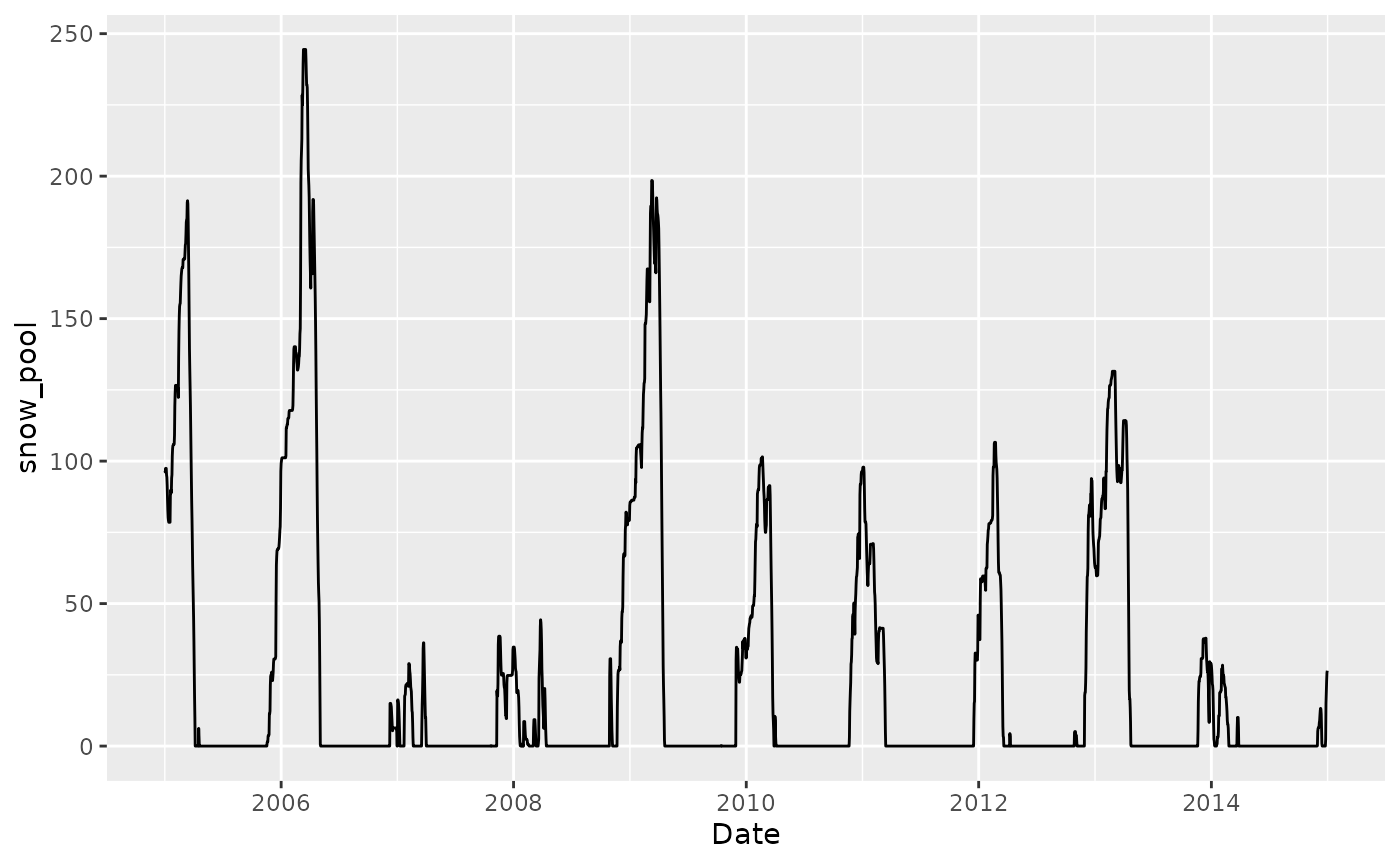
This looks like it’s a lot of snow, actually. Maybe the melting rate is too slow.
Define the daily water balance as liquid water infiltrating into soil (taken as rain plus snow melt) minus evapotranspiration - both in mass units, or equivalently in mm/d.
df <- df |>
  mutate(wbal = liquid_to_soil - et)
Visualise it.
gg5 <- df |>
  ggplot(aes(TIMESTAMP, et)) +
  geom_line()

gg6 <- df |>
  ggplot(aes(TIMESTAMP, liquid_to_soil)) +
  geom_line()

gg7 <- df |>
  ggplot(aes(TIMESTAMP, wbal)) +
  geom_line()

gg5 / gg6 / gg7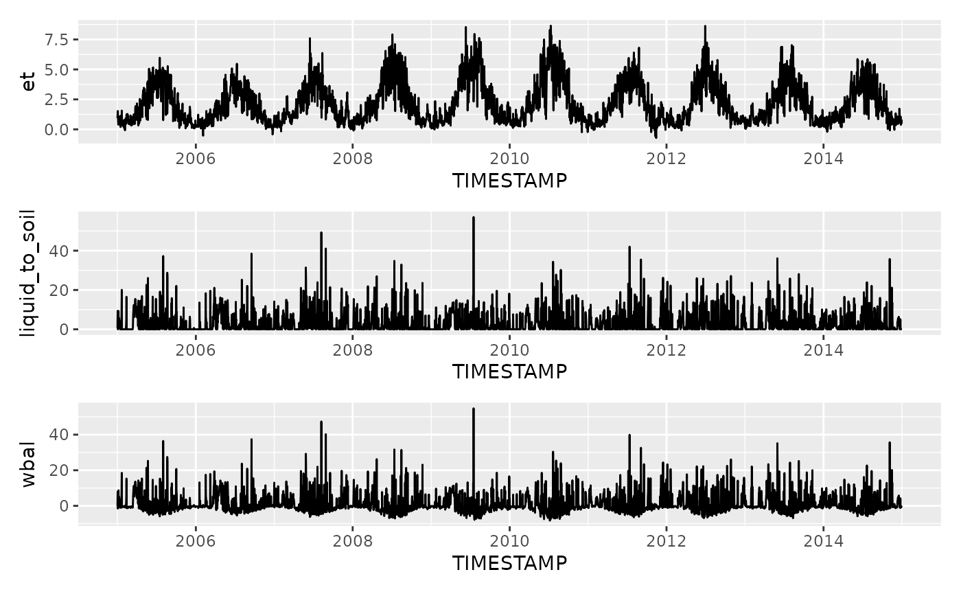
Cumulative water deficit algorithm
Get CWD and events.
out_cwd <- cwd(
  df,
  varname_wbal = "wbal",
  varname_date = "TIMESTAMP",
  thresh_terminate = 0.0,
  thresh_drop = 0.0
  )
Retain only events of a minimum length of 20 days.
out_cwd$inst <- out_cwd$inst |>
  filter(len >= 20)
Plot CWD time series.
ggplot() +
  geom_rect(
    data = out_cwd$inst,
    aes(xmin = date_start, xmax = date_end, ymin = -99, ymax = 99999),
    fill = rgb(0,0,0,0.3),
    color = NA) +
  geom_line(data  =  out_cwd$df, aes(TIMESTAMP, prec), size  =  0.3, color = "royalblue") +
  geom_line(data  =  out_cwd$df, aes(TIMESTAMP, deficit), color = "tomato") +
  coord_cartesian(ylim = c(0, 170)) +
  theme_classic() +
  labs(x = "Date", y = "Cumulative water deficit (mm)")
## Warning: Using `size` aesthetic for lines was deprecated in ggplot2 3.4.0.
## ℹ Please use `linewidth` instead.
## This warning is displayed once per session.
## Call `lifecycle::last_lifecycle_warnings()` to see where this warning was
## generated.
Extreme value statistics
Get annual maxima and fit a general extreme value distribution using the {extRemes} package.
vals <- out_cwd$inst %>%
  group_by(year(date_start)) %>%
  summarise(deficit = max(deficit, na.rm = TRUE)) %>%
  pull(deficit)

evd_gev <- extRemes::fevd(x = vals, type = "GEV", method = "MLE", units = "years")
summary(evd_gev)
##
## extRemes::fevd(x = vals, type = "GEV", method = "MLE", units = "years")
##
## [1] "Estimation Method used: MLE"
##
##
## Negative Log-Likelihood Value: 49.56828
##
##
## Estimated parameters:
## location scale shape
## 84.723272 36.697008 -0.412157
##
## Standard Error Estimates:
## location scale shape
## 13.2609250 10.3279923 0.2916123
##
## Estimated parameter covariance matrix.
## location scale shape
## location 175.852132 -1.605574 -1.80779489
## scale -1.605574 106.667425 -2.10522917
## shape -1.807795 -2.105229 0.08503775
##
## AIC = 105.1366
##
## BIC = 106.0443Get CWD magnitudes for given return periods.
return_period <- c(2, 5, 10, 20, 30, 40, 50, 60, 70, 80, 90, 100, 120, 200, 250, 300, 500, 800)

return_level <- extRemes::return.level(
  evd_gev,
  return.period = return_period
)
df_return <- tibble(
  return_period = return_period,
  return_level = unname(c(return_level)),
  trans_period = -log( -log(1 - 1/return_period)) )

df_return |>
  ggplot(aes(return_period, return_level)) +
  geom_point() +
  labs(x = "Return period (yr)",
       y = "Magnitude of annual CWD maximum (mm)",
       title = "GEV")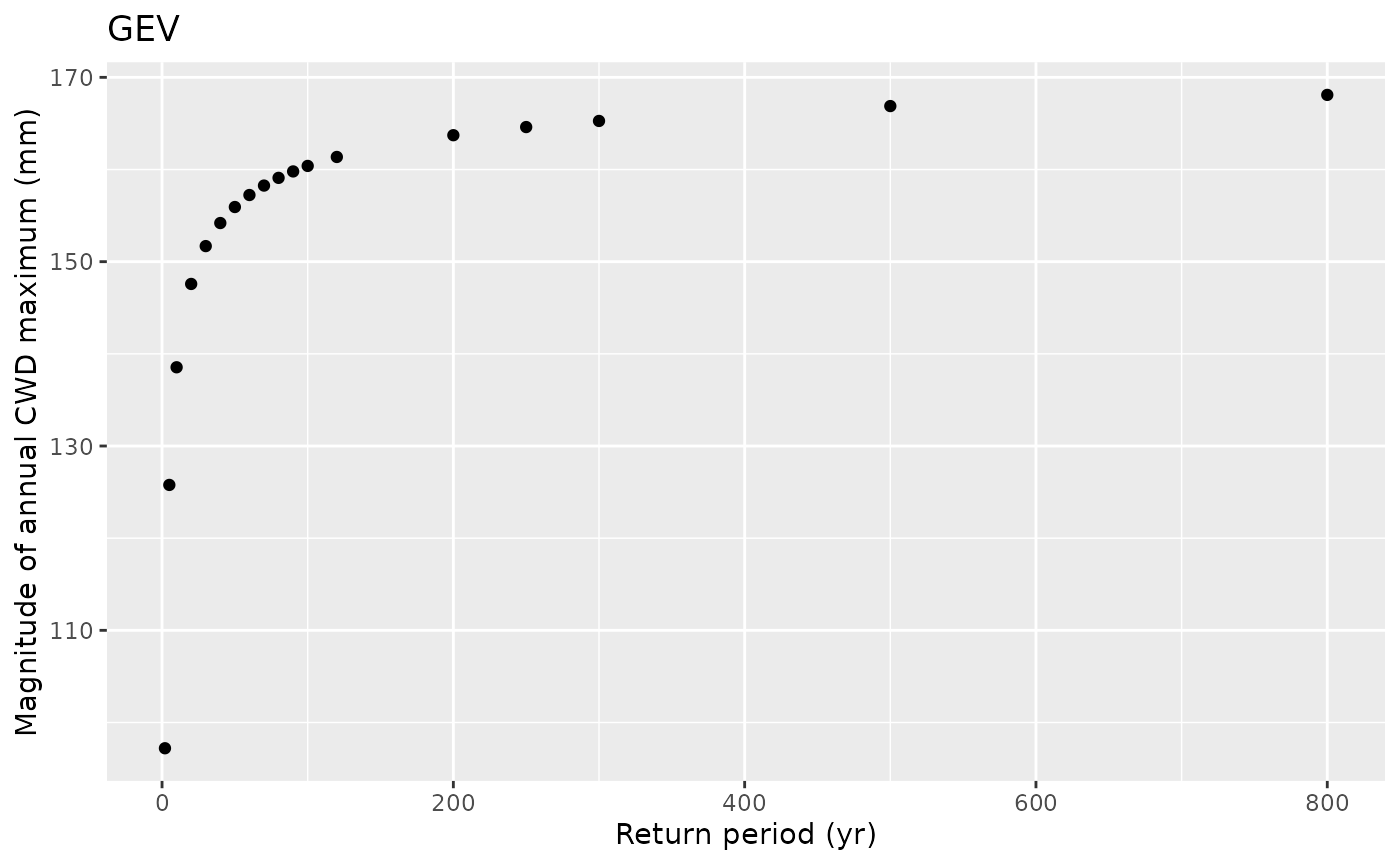
With a Gumbel extreme value distribution, the return period as a function of the CWD extreme magnitude is calculated as follows:
# Fit Gumbel distribution
evd_gumbi <- extRemes::fevd(x = vals, type = "Gumbel", method = "MLE", units = "years")
summary(evd_gumbi)
##
## extRemes::fevd(x = vals, type = "Gumbel", method = "MLE", units = "years")
##
## [1] "Estimation Method used: MLE"
##
##
## Negative Log-Likelihood Value: 50.26535
##
##
## Estimated parameters:
## location scale
## 77.33370 32.62668
##
## Standard Error Estimates:
## location scale
## 10.936112 7.919814
##
## Estimated parameter covariance matrix.
## location scale
## location 119.59854 28.88856
## scale 28.88856 62.72345
##
## AIC = 104.5307
##
## BIC = 105.1359
# calculate return period as a function of the CWD extreme. Using the two
# coefficients of the fitted distribution as arguments
calc_return_period <- function(x, loc, scale){
  1 / (1 - exp(-exp(-(x-loc)/scale)))
}

extract_loc <- function(mod){
  loc <- mod$results$par[ "location" ]
  if (!is.null(loc)){
    return(loc)
  } else {
    return(NA)
  }
}

extract_scale <- function(mod){
  scale <- mod$results$par[ "scale" ]
  if (!is.null(scale)){
    return(scale)
  } else {
    return(NA)
  }
}

# demo return periods
return_period <- c(2, 5, 10, 20, 30, 40, 50, 60, 70, 80, 90, 100, 120, 200, 250, 300, 500, 800)

# use built-in function to get expected CWD extreme for given return periods
# (inverse of probability)
return_level <- extRemes::return.level(
  evd_gumbi,
  return.period = return_period
)

# create data frame for visualisation
df_return <- tibble(
  return_period = return_period,
  return_level = unname(c(return_level)),
  trans_level = -log( -log(1 - 1/return_period))) |>
  mutate(myreturn_period = calc_return_period(
    return_level,
    extract_loc(evd_gumbi),
    extract_scale(evd_gumbi)
  ))

# CWD extreme for a given return period
df_return |>
  ggplot(aes(return_period, return_level)) +
  geom_point() +
  labs(x = "Return period (yr)",
       y = "Magnitude of annual CWD maximum (mm)",
       title = "Gumbel")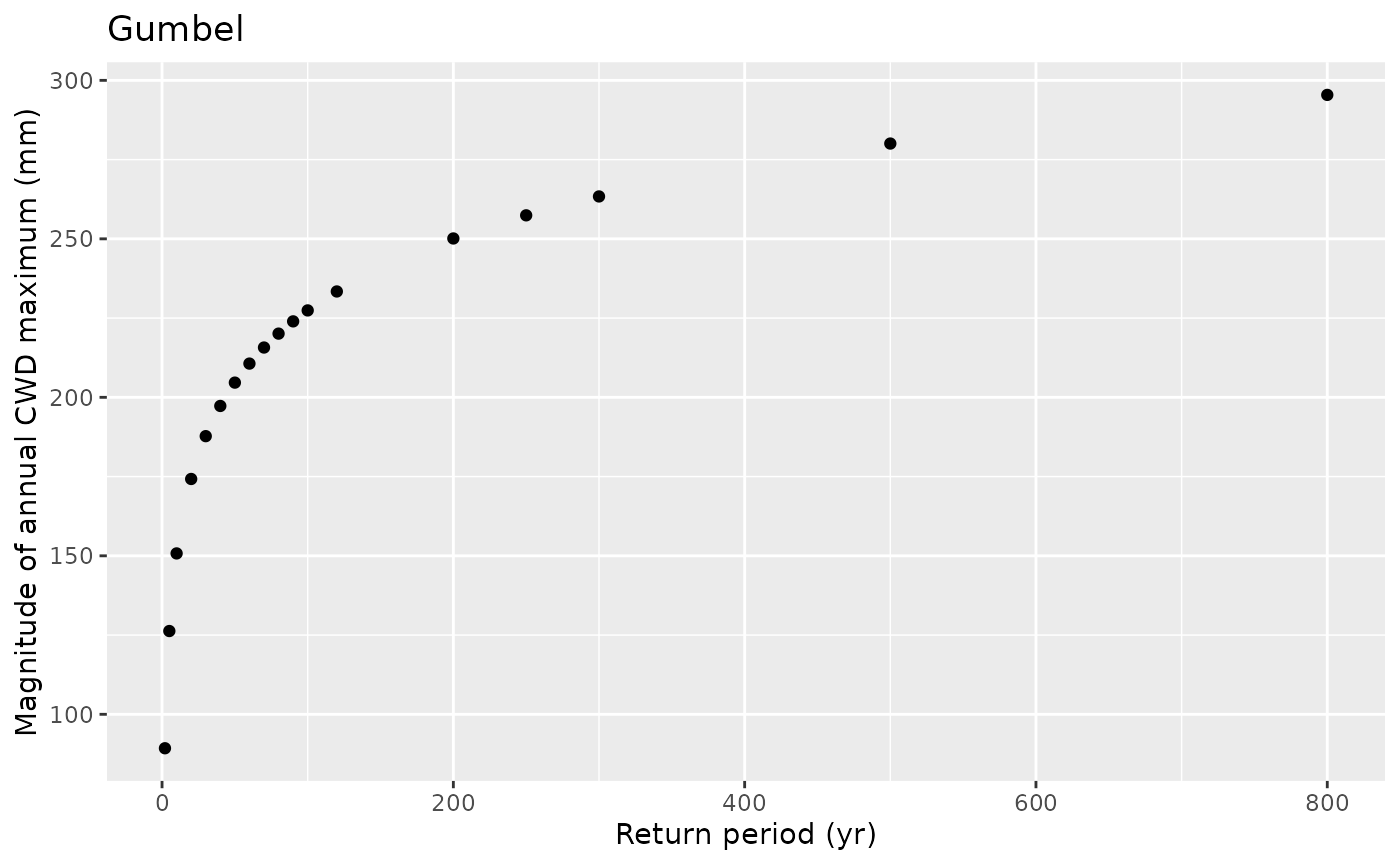
# Return period for a given CWD extreme (calculated based on function above)
df_return |>
  ggplot(aes(return_level, myreturn_period)) +
  geom_point() +
  labs(y = "Return period (yr)",
       x = "Magnitude of annual CWD maximum (mm)",
       title = "Gumbel")
Visualise the estimated event size with a return period of y as the red line on top of the distribution of cumulative water deficit events.
ggplot() +
  geom_histogram(
    data = out_cwd$inst,
    aes(x = deficit, y = after_stat(density)),
    color = "black",
    position="identity",
    bins = 6
    ) +
  labs(x = "Cumulative water deficit (mm)") +
  geom_vline(xintercept = df_return %>%
               dplyr::filter(return_period == 80) %>%
               pull(return_level),
             col = "tomato")
Time stepping
The data frame used above contains time series with daily resolution. The CWD algorithm can also be applied to data provided at other time steps. It primarily acts on the rows in the data frame.
wdf <- df |>
  mutate(year = lubridate::year(TIMESTAMP),
         week = lubridate::week(TIMESTAMP)) |>
  group_by(year, week) |>
  summarise(wbal = sum(wbal, na.rm = FALSE)) |>

  # create a date object again, considering the first day of the week
  mutate(date = lubridate::ymd(paste0(year, "-01-01")) + lubridate::weeks(week-1))
## `summarise()` has regrouped the output.
## ℹ Summaries were computed grouped by year and week.
## ℹ Output is grouped by year.
## ℹ Use `summarise(.groups = "drop_last")` to silence this message.
## ℹ Use `summarise(.by = c(year, week))` for per-operation grouping
## (`?dplyr::dplyr_by`) instead.
out_cwd_weekly <- cwd(wdf,
varname_wbal = "wbal",
varname_date = "date",
thresh_terminate = 0.0,
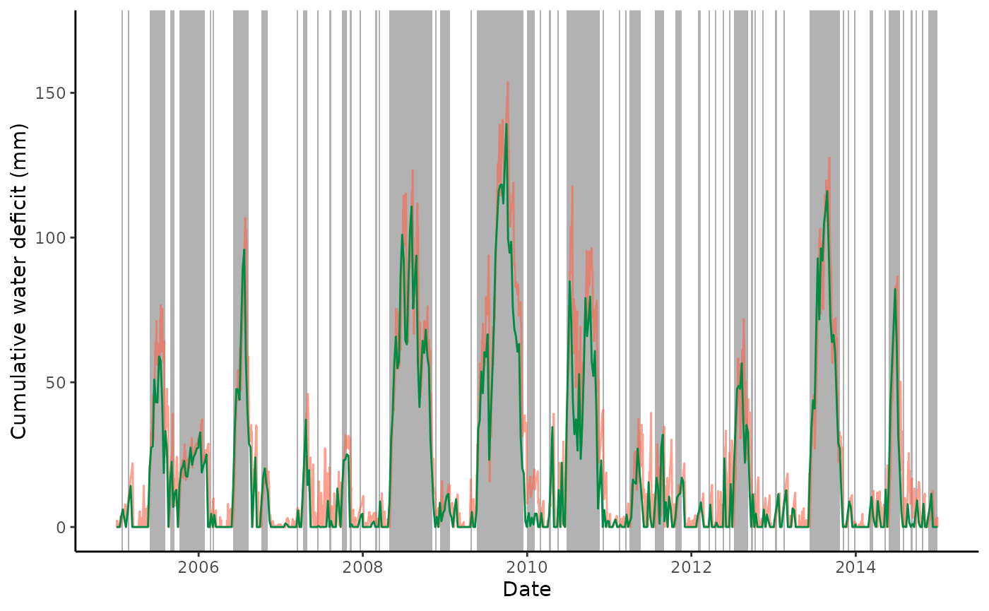
thresh_drop = 0.0)Plot weekly CWD time series in green (Daily CWD time series are plotted by the red line.)
ggplot() +
  geom_rect(
    data = out_cwd_weekly$inst,
    aes(xmin = date_start, xmax = date_end, ymin = -99, ymax = 99999),
    fill = rgb(0,0,0,0.3),
    color = NA) +
  geom_line(data  =  out_cwd$df, aes(TIMESTAMP, deficit), color = "tomato", alpha = 0.6) +
  geom_line(data  =  out_cwd_weekly$df, aes(date, deficit), color = "springgreen4") +
  coord_cartesian(ylim = c(0, 170)) +
  theme_classic() +
  labs(x = "Date", y = "Cumulative water deficit (mm)")