Bern drought monitor

Author

Benjamin Stocker, Fabian Bernhard & Sascha Friedli

Published

July 29, 2026

Overview

This drought monitor combines several complementary variables to assess the current drought situation with a focus on the region of Bern, Switzerland:

  • Potential cumulative water deficit derived from local MeteoSwiss station data and ERA5-Land climate reanalysis.
  • Soil water potential (local measurements by GECO, University of Bern)
  • Tree water deficit (local measurements by GECO, University of Bern)
  • Vegetation Health Index, SwissEO VHI (satellite-derived product by swisstopo)

The combinations of these variables provides insights into the severity of current drought conditions with respect to the atmosphere, the soil, and the vegetation.

Potential cumulative water deficit (PCWD)

NoteExplainer: Potential cumulative water deficit

Potential cumulative water deficit: Measures primarily the meteorological drought condition, but closely reflects soil moisture drying due to its consideration of the balance of water inputs (precipitation) and losses (evapotranspiration). It is calculated as the running sum of potential evapotranspiration (PET) minus precipitation, whereby negative values (water surplus) are not accumulated and reset to zero at each time step (day). Increasing PCWD values indicate progressive soil drying and increasing drought stress of vegetation. Periods with decreasing PCWD indicate conditions where precipitation exceeds PET and reduces and re-wets the rooting zone of vegetation.

PCWD is calculated here from daily precipitation and potential evapotranspiration (PET) data using the cwd::cwd() algorithm (described here). The primary estimate uses MeteoSwiss FAO reference PET. A temperature-based Thornthwaite estimate provides the longer historical context before 1981.

To put current meteorological drought conditions in perspective, we compare potential cumulative water deficit (PCWD) in 2026 against past years. PCWD is derived from temperature and radiation measurements obtained from the MeteoSwiss station Bern/Zollikofen.

PCWD using MeteoSwiss FAO reference evapotranspiration

MeteoSwiss provides daily FAO reference evapotranspiration (erefaod0) for Bern/Zollikofen from 1981 onwards. Using this directly avoids estimating PET from a subset of the station measurements and provides a longer comparison period than radiation-based estimates. The four missing daily FAO PET values in 2006 and 2007 are linearly interpolated from the neighbouring observations.

Code
highlight_colours <- c(
  "2026" = "#D73027",
  "2022" = "#4575B4",
  "2018" = "#E69F00",
  "2023" = "#009E73",
  "1947" = "#CC79A7",
  "1976" = "#56B4E9",
  "2003" = "#F0E442"
)

highlight_years <- as.integer(names(highlight_colours))

meteo_pcwd_FAO_METEOSWISS <- meteo_pcwd |>
  filter(!is.na(PCWD_FAO_MeteoSwiss)) |>
  mutate(plot_date = make_date(2000, month(date), day(date)))

p_fao_meteoswiss <- ggplot() +
  geom_line(
    data = meteo_pcwd_FAO_METEOSWISS |>
      filter(!year %in% highlight_years),
    aes(x = plot_date, y = PCWD_FAO_MeteoSwiss, group = year),
    colour = "grey75",
    linewidth = 0.4,
    alpha = 0.5
  ) +
  geom_line(
    data = meteo_pcwd_FAO_METEOSWISS |>
      filter(year %in% highlight_years),
    aes(
      x = plot_date,
      y = PCWD_FAO_MeteoSwiss,
      colour = as.factor(year),
      group = year
    ),
    linewidth = 0.5
  ) +
  geom_text(
    data = meteo_pcwd_FAO_METEOSWISS |>
      filter(year %in% highlight_years) |>
      group_by(year) |>
      filter(PCWD_FAO_MeteoSwiss == max(PCWD_FAO_MeteoSwiss)) |>
      slice_tail(n = 1) |>
      ungroup(),
    aes(
      x = plot_date,
      y = PCWD_FAO_MeteoSwiss,
      colour = as.factor(year),
      label = year
    ),
    vjust = -0.1,
    show.legend = FALSE
  ) +
  geom_text(
    data = meteo_pcwd_FAO_METEOSWISS |>
      filter(!year %in% highlight_years) |>
      group_by(year) |>
      filter(PCWD_FAO_MeteoSwiss == max(PCWD_FAO_MeteoSwiss)) |>
      slice_tail(n = 1) |>
      ungroup() |>
      arrange(desc(PCWD_FAO_MeteoSwiss)) |>
      slice_head(n = 5),
    aes(x = plot_date, y = PCWD_FAO_MeteoSwiss, label = year),
    vjust = -0.1,
    colour = "grey55",
    show.legend = FALSE
  ) +
  scale_colour_manual(
    values = highlight_colours,
    name = "Year"
  ) +
  scale_x_date(
    date_breaks = "1 month",
    date_labels = "%b"
  ) +
  labs(
    x = NULL,
    y = "PCWD (mm)",
    title = "Potential cumulative water deficit",
    subtitle = paste0(
      "Bern-Zollikofen, MeteoSwiss FAO PET (",
      min(meteo_pcwd_FAO_METEOSWISS$year, na.rm = TRUE),
      "–",
      max(meteo_pcwd_FAO_METEOSWISS$year, na.rm = TRUE),
      ")"
    )
  ) +
  general_plot_theme +
  theme(
    legend.position = "inside",
    legend.position.inside = c(0.01, 1),
    legend.justification = c(0, 1),
    legend.direction = "vertical",
    legend.box = "vertical"
  )

p_fao_meteoswiss
Figure 1: Potential cumulative water deficit in Bern/Zollikofen based on MeteoSwiss FAO reference evapotranspiration.

PCWD of current year vs. long historical context

Potential evapotranspiration may also be estimated from air temperature using the Thornthwaite method. This is less reliable than the MeteoSwiss FAO reference PET, but it extends the comparison back to 1864 and therefore provides a much longer historical context.

Code
meteo_pcwd_THORNTWAITE <- meteo_pcwd |> 
  filter(!is.na(PCWD_THORN)) |>
  mutate(plot_date = make_date(2000, month(date), day(date)))

p_thorn <- ggplot() +
  geom_line(
    data = meteo_pcwd_THORNTWAITE |> filter(!year %in% highlight_years),
    aes(x = plot_date, y = PCWD_THORN, group = year),
    colour = "grey75",
    linewidth = 0.4,
    alpha = 0.5
  ) +
  geom_line(
    data = meteo_pcwd_THORNTWAITE |>  filter(year %in% highlight_years),
    aes(x = plot_date, y = PCWD_THORN, colour = as.factor(year), group = year),
    linewidth = 0.5
  ) +
  # add labels to maximum (first highlight years, then for 5 largest non-highlight years)
  geom_text(data = meteo_pcwd_THORNTWAITE |> filter(year %in% highlight_years) |>
      group_by(year) |>
      # keep only yearly maxima:
      filter(PCWD_THORN == max(PCWD_THORN)),
    aes(x = plot_date, y = PCWD_THORN, colour = as.factor(year), label = year),
    vjust = -0.1, show.legend = FALSE
  ) +
  geom_text(data = meteo_pcwd_THORNTWAITE |> filter(!year %in% highlight_years) |>
      group_by(year) |>
      # keep only yearly maxima:
      filter(PCWD_THORN == max(PCWD_THORN)) |>
      # keep only years among the top 5 maxima
       ungroup() |> arrange(desc(PCWD_THORN)) |> slice(1:5),
    aes(x = plot_date, y = PCWD_THORN, label = year),
    vjust = -0.1, show.legend = FALSE, color = "grey75"
  ) + 
  scale_colour_manual(
    values = highlight_colours,
    name = "Year"
  ) +
  scale_x_date(
    date_breaks = "1 month",
    date_labels = "%b"
  ) +
  labs(
    x = NULL,
    y = "PCWD (mm)",
    title = "Potential cumulative water deficit",
    subtitle = paste0(
      "Bern-Zollikofen, Thornthwaite PET (",
      min(meteo_pcwd_THORNTWAITE$year, na.rm = TRUE), "–", max(meteo_pcwd_THORNTWAITE$year, na.rm = TRUE), ")"
    )
  ) +
  general_plot_theme +
  theme(
    legend.position = "inside", legend.position.inside = c(0.01,1),  legend.justification = c(0,1),
    legend.direction = "vertical", legend.box = "vertical"
  )

p_thorn

# ggsave(
#   here("fig", "pcwd_thorntwaite.pdf"),
#   width = 8,
#   height = 5
# )
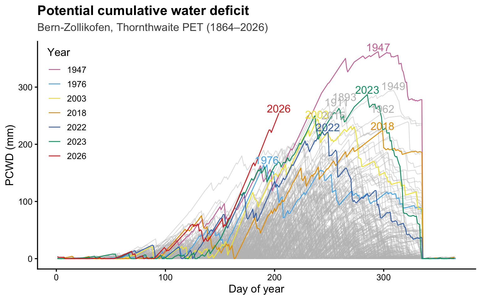
Figure 2: Potential cumulative water deficit in Bern/Zollikofen based on Thornthwaite PET using the full available temperature record.

Finding

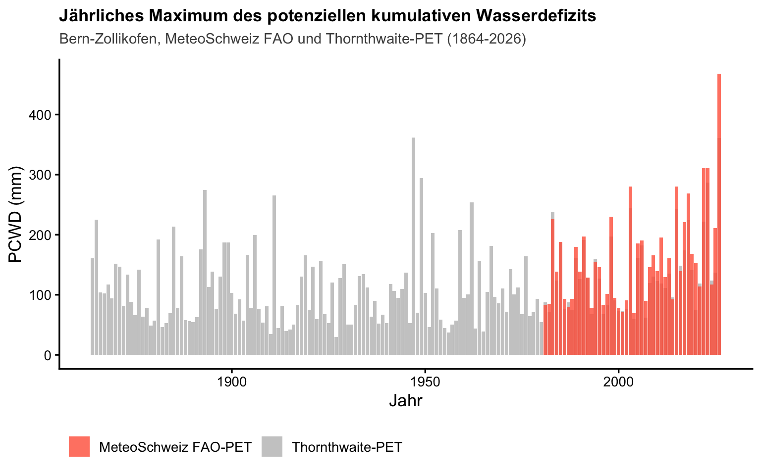
The historical drought year of 1947 featured even higher PCWD than are currently attained in 2026. However, given the timing in the season, 2026 stands out as (by far) unprecedented. In no other years since measurements began did the PCWD attain such high values by mid-July as in 2026. Given that the PCWD typically continues rising in throughout August and Septempter, it is to be expected that the 1947 record PCWD (then attained in fall) will be broken.

Note that the temperature-only Thornthwaite method yields somewhat different results from PCWD based on MeteoSwiss FAO reference evapotranspiration. The FAO-based result should therefore be preferred where it is available; Thornthwaite is retained to provide context before 1981.

Spatial visualisation of current PCWD

To illustrate the current spatial distribution across Switzerland, we additionally show PCWD from the global ERA5-Land climate reanalysis dataset for the ongoing year. This spatial product uses Priestley–Taylor PET; it is separate from the station-based year-comparison series above.

The map shows the spatial distribution of PCWD across Switzerland at the indicated date, with the regional temporal evolution shown by the inset.

Code
# laad data for ERA5-Land map and ERA5-Land timeseries
cwd_ERA5Land <- terra::rast(
  here("data/ERA5LandCWD/data_derived_03_daily_pcwd_v2-doy_2026_r-generated_regionCH.nc") # or "regionBern.nc" or "regionEUROPE.nc"
)
cwd_ERA5Land_df <- dplyr::bind_rows(
  tidync::hyper_tibble(here("data/ERA5LandCWD/data_derived_03_daily_pcwd_v2-doy_2026_r-generated_regionCH.nc")), # or "regionBern.nc" or "regionEUROPE.nc"
  tidync::hyper_tibble(here("data/ERA5LandCWD/data_derived_03_daily_pcwd_v2-doy_2025_r-generated_regionCH.nc")), # or "regionBern.nc" or "regionEUROPE.nc"
) |> mutate(time = lubridate::ymd(time))

# plot ERA5-Land map
date_to_plot <- "2026-07-15"
raster_to_plot_ERA5LAND_PCWD <- cwd_ERA5Land[[time(cwd_ERA5Land) %in% date_to_plot]]

# Define similar palette to vhi:
# CONTINUOUS PALETTE:
# pal_ERA5LAND_PCWD <- colorNumeric(
#   #palette = "viridis",
#   palette = rev(vhi_cols),
#   domain = values(raster_to_plot_ERA5LAND_PCWD),
#   na.color = "transparent"
# )
# Discretized PALETTE:
pal_ERA5LAND_PCWD <- colorBin(
  palette = rev(vhi_cols),
  domain = values(raster_to_plot_ERA5LAND_PCWD),
  bins = 15,
  na.color = "transparent"
)

# Prepare the regional average time series plot (will be embedded into the map)
cwd_ERA5Land_df_mean <- cwd_ERA5Land_df |> 
  group_by(time) |> summarise(pcwd_mm = mean(pcwd_mm)) |> 
  slice_head(n = -1) # drop last line which appears to be set to pcwd_mm = 0

plt_ERA5Land_temp <- ggplot(cwd_ERA5Land_df_mean, aes(x = time, y=pcwd_mm)) +
  geom_line() + 
  theme_bw() + 
  labs(x=NULL, y= "Region average of PCWD (mm)") + 
  geom_vline(xintercept = ymd(date_to_plot), color = "red") +
  scale_x_date(NULL, date_breaks = "2 month", date_minor_breaks = "1 month", date_labels = "%b") + # \n%Y
  geom_text(data = \(df) slice(df, 1),  # this forces annotation only once
            x = ymd(date_to_plot), y = Inf, 
            label = "Map\ndate", color = "red", vjust=1.2, hjust = -0.5, angle = 270) + # vjust=-0.2
  general_plot_theme

# render the plot to a PNG and encode as data URI for embedding as inset into map
tmp_png <- tempfile(fileext = ".png")
ggsave(filename = tmp_png, plot = plt_ERA5Land_temp + labs(y=NULL),
       width = 600, height = 220, units = "px", dpi = 150)
img_uri <- base64enc::dataURI(file = tmp_png, mime = "image/png")

# generate map as leaflet
leaflet() |>
  addMapPane("basemap", zIndex = 1) |> # NOTE: pane is a fix to better control order
  addProviderTiles(providers$SwissFederalGeoportal.NationalMapGrey, group = "swisstopo Topo",       options = providerTileOptions(opacity = 1.0, pane = "basemap")) |>
  addProviderTiles(providers$SwissFederalGeoportal.SWISSIMAGE,      group = "swisstopo SWISSIMAGE", options = providerTileOptions(opacity = 1.0, pane = "basemap")) |>
  addProviderTiles(providers$Stadia.StamenTonerLite,                group = "Stamen Greyscale",     options = providerTileOptions(opacity = 1.0, pane = "basemap")) |>
  addLayersControl(
    baseGroups = c("swisstopo Topo", "swisstopo SWISSIMAGE", "Stamen Greyscale", "No background"),
    overlayGroups = c(sprintf("ERA5-Land PCWD (%s)", date_to_plot)),
    position = "topleft",
    options = layersControlOptions(collapsed = FALSE)
  ) |>
  # add inset image:
  addControl(
    position = "topleft",
    html = paste0("<style>
                  .leaflet-control-layers { width:220px !important; box-sizing:border-box; }
                  </style>", 
                  sprintf(
                    "<div style='width:%dpx;background:rgba(255,255,255,0.95);border-radius:4px;'><strong>Region average PCWD (mm)</strong><br/><img src='%s' style='width:100%%;height:auto;display:block;'/></div>",
      220-16, img_uri)) # 220px - 2*8px padding
  ) |>
  # add main raster image:
  addRasterImage(
    raster_to_plot_ERA5LAND_PCWD,
    colors = pal_ERA5LAND_PCWD,
    opacity = 0.75,
    group = sprintf("ERA5-Land PCWD (%s)", date_to_plot),
    attribution = paste(
      "\n&copy; Copernicus Climate Change Service information (2019). Muñoz Sabater, J. (2019): ERA5-Land hourly data from 1950 to present. Copernicus Climate Change Service (C3S) Climate Data Store (CDS). DOI: 10.24381/cds.e2161bac (Accessed on 16-Jul-2026) Generated using or contains modified Copernicus Climate Change Service information <2019>. Neither the European Commission nor ECMWF is responsible for any use that may be made of the Copernicus information or data it contains."
    )
  ) |>
  addLegend(
    position = "topright",
    pal = pal_ERA5LAND_PCWD, 
    values = values(raster_to_plot_ERA5LAND_PCWD), 
    opacity = 1,
    title = "PCWD (mm)"
  )
Figure 3: Potential cumulative water deficit across central Europe on 2026-07-15 from ERA5-Land reanalysis data (using Priestley Taylor PET).

Finding

PCWD is not evenly distributed across Switzerland. The highest values are attained around Zurich, Zürcher Unterland, Schaffhausen, Basel, Lausanne, and the southern tip of Ticino. Across the Prealps and main ridge of the Alps, PCWD is substantially lower.

ERA5-Land precipitation, an input to PCWD, may be less reliable in mountain regions. This likely contributes to the low modelled PCWD in the Rhône valley despite documented dryness there.

Soil water potential

NoteExplainer: Soil water potential

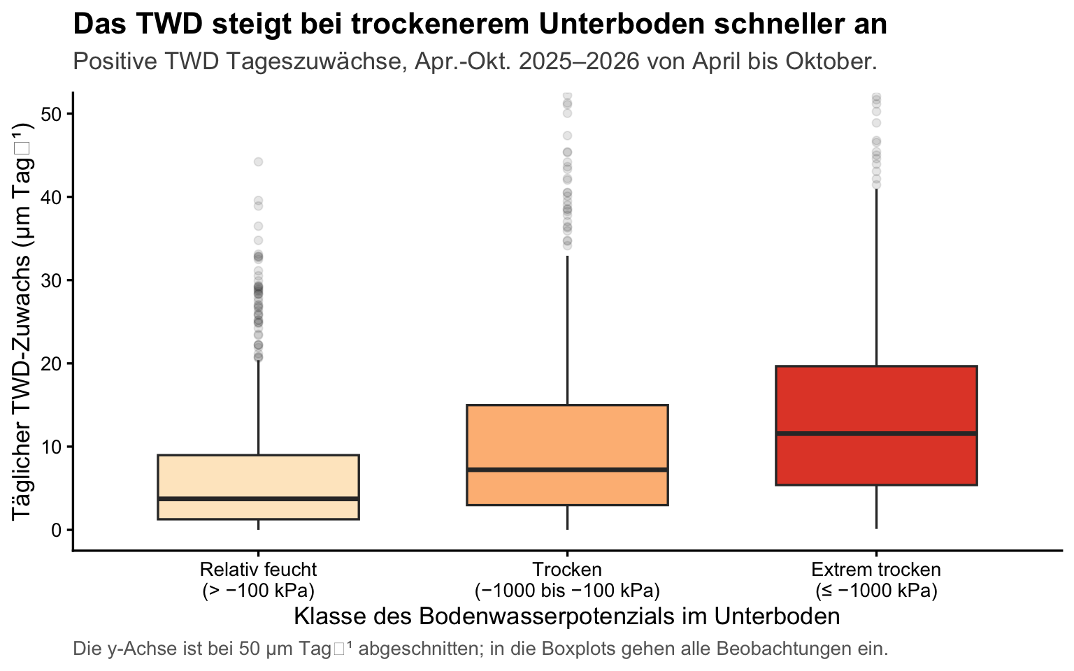
Measures soil moisture drought in pressure units. In contrast to soil water content in mass or volumetric units, the soil water potential measures the force plants have to overcome to extract water from the soil matrix. It is therefore closely reflective of the physiological effects of water stress a plant is exposed to.

Soil water potentials are measured along a forested hillslope near Bern, stretching from an area adjacent to the river Aare to an elevated (flat) position ca. 80 m above the river. The three positions (high, mid and low in plots below) indicate the height above the Aare river–the neareast drainage channel.

The measurement campaign was started in 2025 and is supported by the Burgergemeinde Bern, and Dr. Roman Zweifel (WSL, Birmensdorf) through the UPSCALE project.

Code
df_SWP_plot <- df_SWP |>
  mutate(
    year = factor(
      lubridate::year(date),
      levels = c(2025, 2026)
    ),

    # Map 2025 and 2026 onto the same reference year
    # so that the seasonal trajectories can be compared directly
    plot_date = as.Date(
      sprintf(
        "2000-%02d-%02d",
        lubridate::month(date),
        lubridate::day(date)
      )
    ),

    depth = factor(
      series_height,
      levels = c(-0.1, -0.4, -0.6, -1),
      labels = c("10 cm", "40 cm", "60 cm", "100 cm")
    ),

    # Keep the desired panel order
    plot = factor(
      tree_name,
      levels = c("P3", "P2", "P1", "G1"), labels = c("High","Mid","Low", "G1")
    )
  ) |>
  filter(
    year %in% c("2025", "2026"),
    plot %in% c("High","Mid","Low"),
    !is.na(SWP_mean),
    !is.na(depth)
  )

p1 <- 
  ggplot(
    df_SWP_plot,
    aes(
      x = plot_date,
      y = SWP_mean,
      colour = year,
    )
  ) +
  geom_line(
    linewidth = 0.7,
    alpha = 0.9,
    na.rm = TRUE
  ) +
  facet_grid(
    cols = vars(plot),
    rows = vars(depth),
    scales = "fixed",
    labeller = labeller(depth = label_both,
                        .default = label_value)
  ) +
  scale_colour_manual(
    values = c(highlight_colours, c("2025" = "darkgrey")),
    drop = FALSE
  ) +
  scale_x_date(
    date_breaks = "2 month",
    date_minor_breaks = "1 month",
    date_labels = "%b",
    limits = as.Date(c("2000-01-01", "2000-12-31")),
    expand = expansion(mult = c(0.01, 0.01))
  ) +
  scale_y_continuous() + 
  labs(
    title = "Seasonal dynamics of soil water potential",
    x = NULL,
    y = "Soil water potential (kPa)",
    colour = NULL,
    caption = paste(
      "More negative values indicate drier soil conditions."
    )
  ) +
  general_plot_theme +
  theme(
    legend.position = "inside", legend.position.inside = c(0.01,0.01),  legend.justification = c(0,0),
    legend.direction = "vertical", legend.box = "vertical"
  )

p1
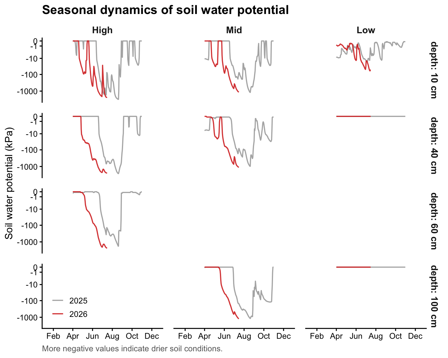
Figure 4: Seasonal dynamics of soil water potential at different landscape positions (above Aare river) and soil depths in 2025 and 2026.

Finding

The soil has dried out much earlier in 2026 than in 2025. The current levels of the soil water potential (low values indicate dry conditions) are of similar magnitude as the driest values in 2025. However, in 2025, low values were attained much later in the season.

Interestingly, the mid and especially the low position experience generally less negative soil water potentials than the high position. In other words, the higher above the Aare river, the drier the soil gets over the course of a summer. This may be due to lateral water transport along the hillslope and the influence of the river, leading to shallow groundwater tables in the low position–likely within the reach of tree roots. Tree water use can also be different with soil depth depending on the root distributions. Typically, deeper soil layers remain wetter due to reduced root water uptake. However, in the above measurements the main dry-out of the soil in 2025 and 2026 was similar across all soil depths (except for the position close to the Aare).

Tree water deficit

NoteExplainer: Tree water deficit

Measures the actual water stress experienced by a tree. Derived from the daily swelling (during the night) and contraction (during the day) of the trunk. Anomalously small swelling and strong contraction yields a high tree water deficit and is indicative of low water availability in the rooting zone of the respective tree. The advantange of tree water deficit measurements over soil water potential measurements is that they naturally integrate over the actual rooting zone of the tree, while soil water potential measurements are only indicative of conditions at the soil depth where the sensor is placed.

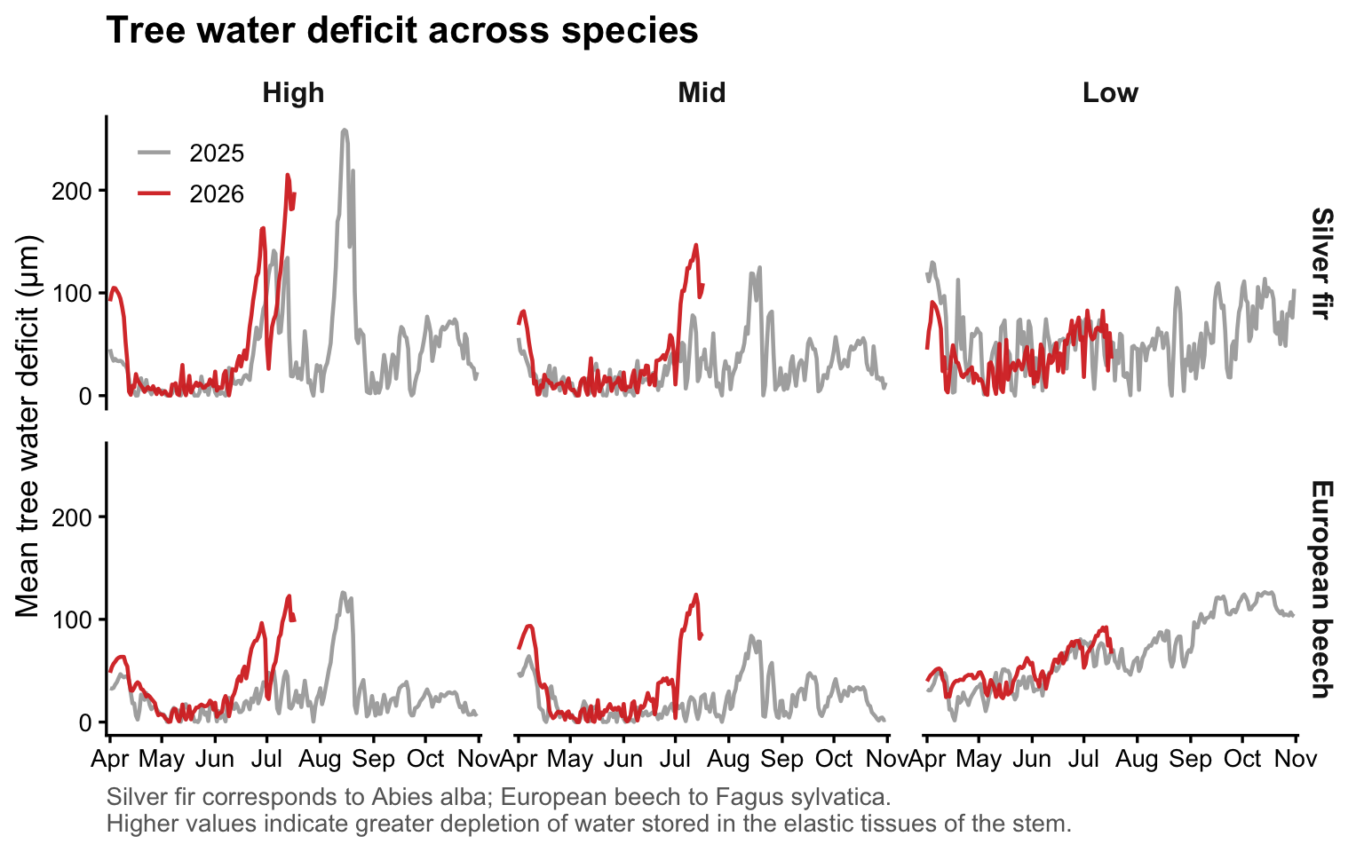
As part of the same campaign as for the soil water potential measurements (see above), also tree water deficits were measured in the same positions. The three positions (high, mid and low in plots below) indicate the height above the Aare river–the neareast drainage channel. Measurements are distinguished for two species (Silver fir and European beech) because responses to water stress are highly species-dependent.

Code
df_TWD_blog <- df_TWD |>
  mutate(
    # Year used for colouring
    year = factor(
      lubridate::year(date),
      levels = c(2025, 2026)
    ),

    # Place both years on the same seasonal x-axis
    plot_date = as.Date(
      sprintf(
        "2000-%02d-%02d",
        lubridate::month(date),
        lubridate::day(date)
      )
    ),

    # Extract site identifier from tree name
    site = stringr::str_sub(tree_name, -2, -1),

    # Define landscape-position labels and order
    plot = factor(
      site,
      levels = c("P3", "P2", "P1", "G1"),
      labels = c("High", "Mid", "Low", "G1")
    ),

    # Short common names for facet labels
    species = factor(
      tree_genus_species,
      levels = c(
        "Abies alba",
        "Fagus sylvatica"
      ),
      labels = c(
        "Silver fir",
        "European beech"
      )
    )
  ) |>
  filter(
    year %in% c("2025", "2026"),
    plot %in% c("High", "Mid", "Low"),
    tree_genus_species %in% c(
      "Abies alba",
      "Fagus sylvatica"
    ),
    lubridate::month(date) >= 4,
    lubridate::month(date) <= 10
  ) |>

  # Keep every individual tree separate
  group_by(
    plot_date,
    year,
    tree_name,
    plot,
    species
  ) |>
  summarise(
    TWD = mean(TWD_mean, na.rm = TRUE),
    .groups = "drop"
  ) |>
  filter(
    is.finite(TWD)
  )


p_twd_blog <- ggplot(
  df_TWD_blog,
  aes(
    x = plot_date,
    y = TWD,
    colour = year,

    # Separate line for every tree and year
    group = interaction(year, tree_name)
  )
) +
  geom_line(
    linewidth = 0.55,
    alpha = 0.55,
    na.rm = TRUE
  ) +

  # Landscape position in rows, species in columns
  facet_grid(
    cols = vars(plot),
    rows = vars(species),
    scales = "fixed"
  ) +

  scale_colour_manual(
    values = c(
      "2025" = "darkgrey",
      "2026" = highlight_colours[["2026"]]
    ),
    drop = FALSE
  ) +

  scale_x_date(
    limits = as.Date(
      c("2000-04-01", "2000-10-31")
    ),
    date_breaks = "1 month",
    date_labels = "%b",
    expand = expansion(
      mult = c(0.01, 0.01)
    )
  ) +

  labs(
    title = "Tree water deficit across individual trees",
    x = NULL,
    y = "Tree water deficit (\u00b5m)",
    colour = NULL,
    caption = paste(
      "Each line represents an individual tree.",
      "Silver fir corresponds to Abies alba; European beech to Fagus sylvatica.\n",
      "Higher values indicate greater depletion of water stored in",
      "the elastic tissues of the stem."
    )
  ) +

  guides(
    colour = guide_legend(
      order = 1
    )
  ) +

  general_plot_theme +

  theme(
    legend.position = "inside",
    legend.position.inside = c(0.01, 1.0),
    legend.justification = c(0, 1),
    legend.direction = "vertical",
    legend.box = "vertical"
  )


p_twd_blog
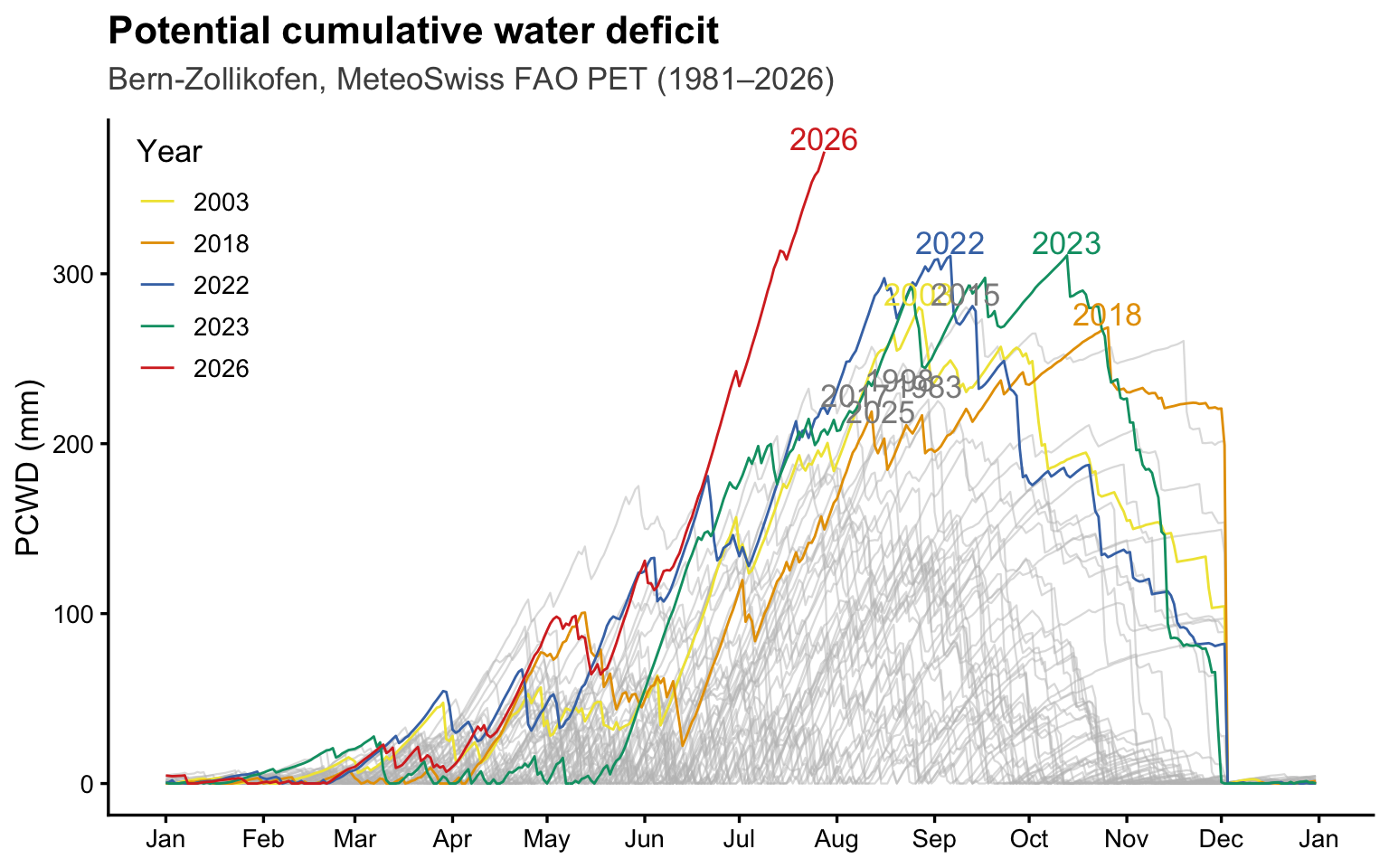
Figure 5: Seasonal dynamics of tree water deficit at different landscape positions (above Aare river) in 2025 and 2026.

Finding

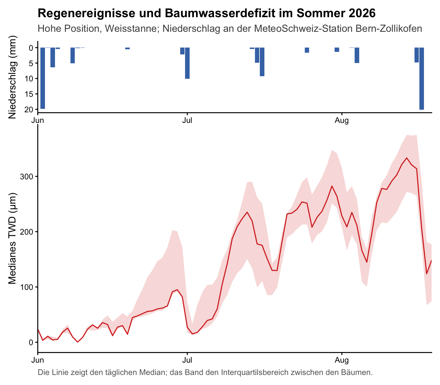
Tree water deficits are as high or higher than ever recorded in 2025. However, in contrast to 2026, deficits have started rising much earlier. This indicates that water stress is has been affecting trees throughout almost the full growing season this year. In contrast, water stress effects at the high and mid positions were limited to August in 2025. This likely has important negative consequences for the carbon balance and growth of trees in 2026.

The low position appears to be almost fully buffered against drought impacts in both years.

Vegetation Health Index (VHI)

NoteExplainer: Vegetation Health Index

Measures impacts of drought on vegetation health, that is greenness and its activity (transpiration). The SwissEO Vegetation Health Index (VHI) combines Sentinel-2-derived Normalised Difference Vegetation Index (NDVI) observations with with land surface temperature (LST) data to provide an indication of vegetation stress. The index ranges from 0 to 100, where lower values indicate less healthy vegetation and a higher likelihood of drought-related impacts. LST reflects vegetation activity as transpiration cools the surface and hence a high land surface temperature can indicate low transpiration rates and hence vegetation water stress. The advantage of this satellite-derived index is that it naturally captures conditions across space. The disadvantage is that it is affected by larger noise in observations, limiting its reliability and interpretability.

The map below shows the most recent VHI data available for the region around Bern region (2026-07-24 (latest valid available)). The median VHI across the study area was 43, with values ranging from 0 to 100.This suggests that vegetation is experiencing noticeable stress. With the warm current temperature the VHI is likely to further decrease over the coming days.

Code
pal_vhi <- colorBin(
  palette = vhi_cols,
  domain = terra::values(vhi_rast_wgs84),
  bins = vhi_bins,
  na.color = "transparent",
  right = FALSE
)

raster_groups <- paste0("VHI ", time(vhi_rast_wgs84))

vhi_map <- leaflet() |>
  addMapPane("basemap", zIndex = 1) |> # NOTE: pane is a fix to better control order
  addProviderTiles(providers$SwissFederalGeoportal.NationalMapGrey, group = "swisstopo Topo",       options = providerTileOptions(opacity = 1.0, pane = "basemap")) |>
  addProviderTiles(providers$SwissFederalGeoportal.SWISSIMAGE,      group = "swisstopo SWISSIMAGE", options = providerTileOptions(opacity = 1.0, pane = "basemap")) |>
  addProviderTiles(providers$Stadia.StamenTonerLite,                group = "Stamen Greyscale",     options = providerTileOptions(opacity = 1.0, pane = "basemap")) |>
  addLayersControl(
    baseGroups = c("No background", "swisstopo Topo", "swisstopo SWISSIMAGE", "Stamen Greyscale"),
    overlayGroups = raster_groups,
    position = "topleft",
    options = layersControlOptions(collapsed = FALSE)
  ) 

for (i in seq_along(raster_groups)){
  vhi_map <- vhi_map |>
    addRasterImage(
      vhi_rast_wgs84[[i]],
      colors = pal_vhi,
      opacity = 1.0, # 0.75 # since VHI map is only forested areas we can easily use 1.0
      group = raster_groups[i],
      attribution = paste(
        "VHI layer: \n&copy; swisstopo, Contains modified Copernicus Sentinel data 2026"
      )
    )
}

vhi_map <- vhi_map |>
  hideGroup(raster_groups[-1]) |>
  showGroup(raster_groups[1]) |>
  addLegend(
    position = "bottomright",
    colors = vhi_cols,
    opacity = 1,
    labels = c(
      "0–9: Extremely stressed",
      "10–19: Very stressed",
      "20–29: Stressed",
      "30–39: Slightly stressed",
      "40–49: Normal",
      "50–59: Good",
      "60–100: Excellent"
    ),
    title = "VHI"
  )
vhi_map
Figure 6: Latest swissEO Vegetation Health Index around Bern (dating from 2026-07-24 (latest valid available) ).

Finding

Extremely stressed vegetation dominates throughout the region. Variability in stress levels should be interpreted with caution. Error sources such as clouds can potentially lead to anomalous values for certain dates.

Current drought status summary

Taken together, the different indicators paint a consistent picture. Spring and early summer of 2026 were characterized by increasing atmospheric water demand and below-average moisture availability. Compared to 2025, these drought indicators increased earlier than 2025.

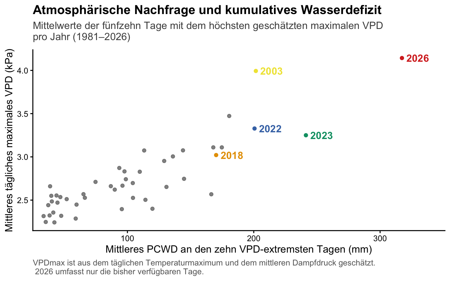
This signal is reflected in the satellite-based Vegetation Health Index, which shows widespread moderate vegetation stress around Bern. At the same time, the PCWD is currently as high as it has ever been at this point in the year.

Both indices indicate that the ecosystem is currently in a state of elevated drought stress. The evolution over the coming weeks will largely depend on the weather in the upcoming weeks. Currently, MeteoSwiss predicts warm temperatures and only little precipitation in the form of thunderstroms over the coming days, which will likely further increase drought stress. Drought levels attained this summer are likely among the highest or are record-breaking with respect to previously recorded values since measurements began (1864).